3.3.2 - Marketing data and forecasts

Graphs and correlation

A graph makes a pattern easier to recognise when its form, labels and scales match the question being investigated.

Use a bar chart to compare categories, such as sales through shops, websites and wholesalers. Put the categories on one axis and the measured value with its units on the other; separate bars make clear that these are distinct groups. A line graph is useful for an ordered sequence such as monthly sales: put time horizontally, sales vertically and join observations in their time order. A pie chart shows how a total is divided, so its categories must be mutually exclusive and add to the whole. A channel accounting for 25% of annual sales occupies $0.25\times360=90$ degrees. The pie chart cannot show growth on its own.

To construct a graph, choose a meaningful title, label both axes, use consistent intervals and plot values accurately. Show any axis break clearly. A vertical scale starting at £99,000 rather than zero can make a rise from £100,000 to £102,000 look dramatic; examine the actual values before judging the business effect. Compare like periods: a three-month sales total and a one-month total are not directly comparable.

A scatter diagram plots pairs of observations for two numerical variables. To compare weekly advertising spending and sales, use one point for each week: spending goes horizontally and sales vertically. Unlike a time-series line, the points should not be joined in date order. A line of best fit, where appropriate, summarises the relationship rather than passing through every observation.

Constructing a time-series graph

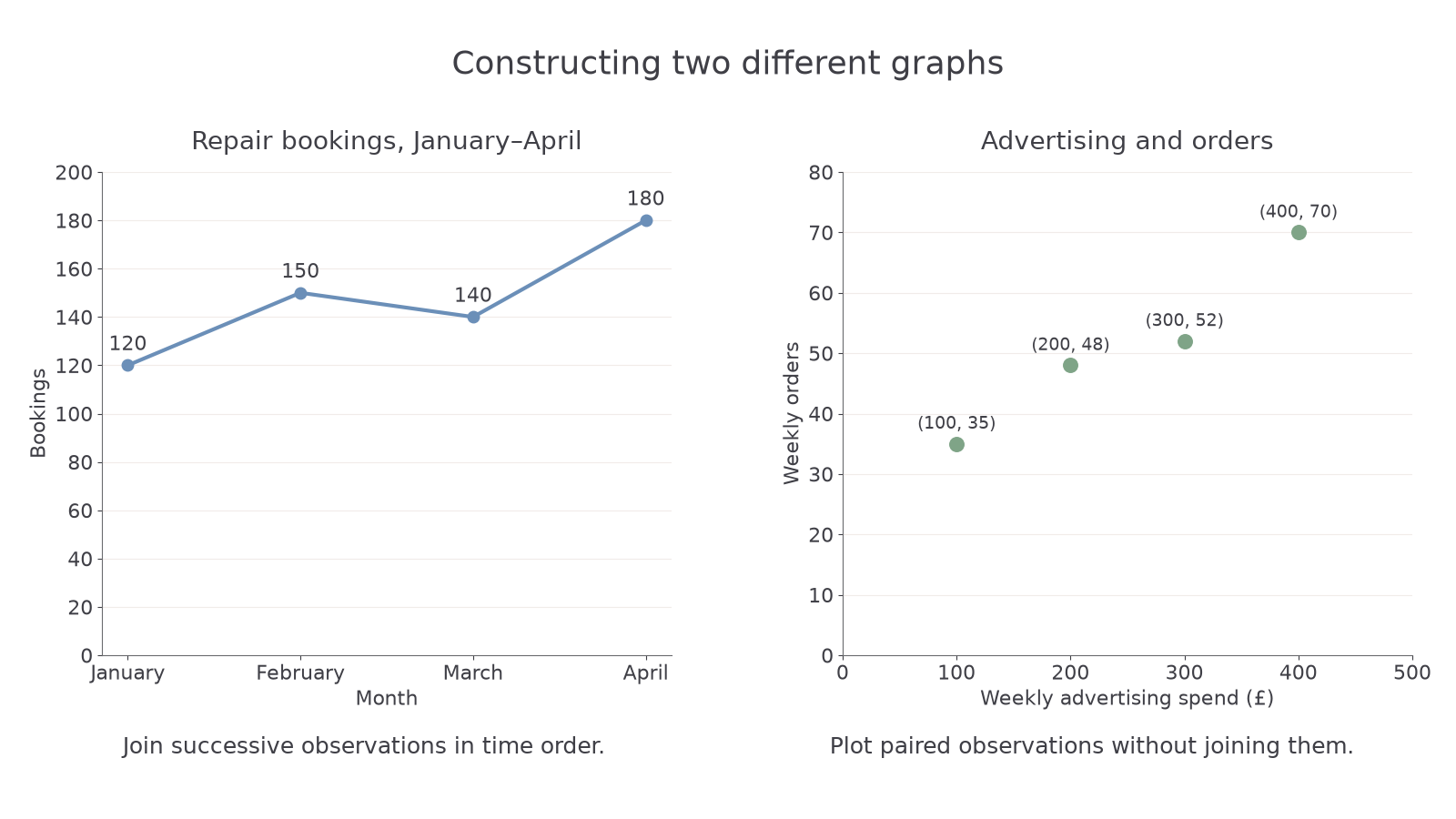
A repair service records monthly bookings of 120 in January, 150 in February, 140 in March and 180 in April.

1. Put the four months in order on the horizontal axis and bookings on the vertical axis, with equal 20-booking intervals from 0 to 200.
2. Plot the coordinates:

1. Join successive months with straight segments. The fall from February to March must remain visible; a smooth rising curve would misrepresent the data.
2. Title the graph “Repair bookings, January–April”. A bar chart could also compare these months, but the connected line emphasises their sequence.

Constructing a scatter diagram

A second firm records four weeks of advertising spend in pounds and orders as paired observations: (100,35), (200,48), (300,52) and (400,70).

1. Label advertising spend horizontally from £0 to £500 and orders vertically from 0 to 80, using constant intervals.
2. Plot one point for each pair:

1. Leave the points unjoined. Their overall upward tendency indicates positive correlation; the scatter means orders do not follow an exact fixed increase.
2. If adding a best-fit line, place it through the central tendency rather than force it through all points. Four observations provide limited evidence about the relationship.

[DIAGRAM: asset_name: Constructing time-series and scatter graphs; asset_slug: business-graph-construction; caption: A time series joins observations in month order, while a scatter diagram leaves each paired observation separate.; description: Left panel shows repair bookings at January 120, February 150, March 140 and April 180, with bookings from zero to 200 and observations joined in time order. Right panel plots advertising pounds and orders at 100 and 35, 200 and 48, 300 and 52, 400 and 70, with separate points and axes beginning at zero. Both datasets are original classroom examples.]

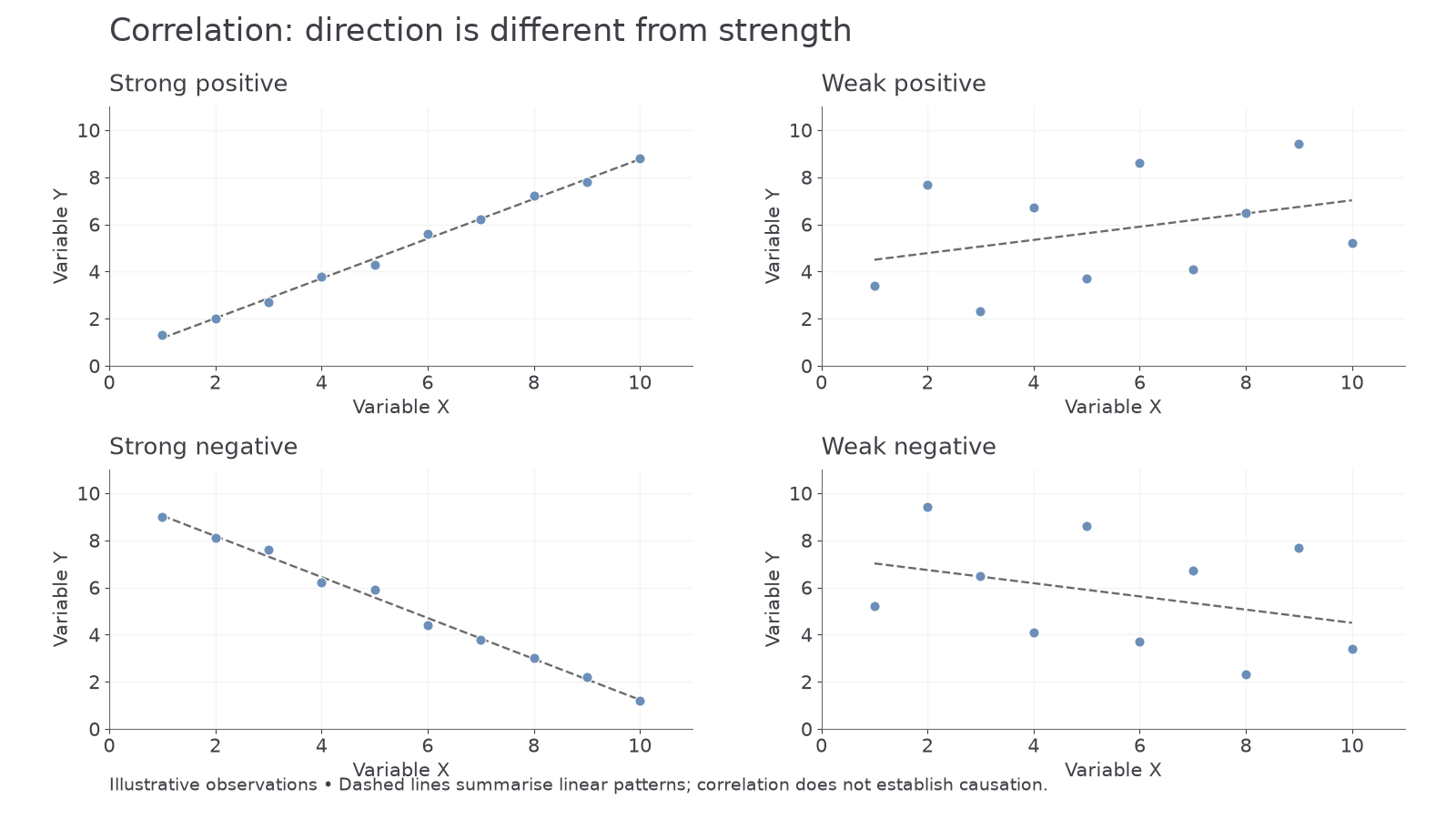
Positive correlation means higher values of one variable tend to occur with higher values of the other. Negative correlation means higher values of one tend to occur with lower values of the other. Strength concerns how closely points follow a relationship, not how steep the line is. Points tightly clustered around an upward line show strong positive correlation; widely scattered points with a slight upward tendency show weaker positive correlation. The same distinction applies to downward patterns. No clear upward or downward pattern suggests little linear correlation, though a curved relationship may still exist.

[DIAGRAM: asset_name: Direction and strength of correlation; asset_slug: aqa_b12_correlation; caption: Direction describes whether variables move together or oppositely, while strength describes how closely the points follow the pattern.; description: Four scatter diagrams share the same numbered scales and show strong positive, weak positive, strong negative and weak negative relationships. Axes represent variable X and variable Y.]

Correlation is not proof of causation. Advertising and sales may rise together because an approaching holiday increases both demand and the firm's advertising budget. Sales success may also give the firm money to advertise, reversing the assumed causal direction. A plausible mechanism, consideration of other variables and better-designed comparisons are needed before claiming that one factor caused the change.

The ONS release of 25 July 2025 estimated Great Britain's retail sales volume rose 0.9% in June after falling 2.8% in May. The series measures quantity bought and uses seasonal adjustment. A business interpreting the graph must preserve that definition and use multiple months; June's rise alone does not establish a sustained recovery or higher sales value. ONS retail sales, June 2025.

Confidence intervals and uncertainty

A sample estimate can be useful while still differing from the true value in the population.

A confidence interval gives a range produced by a statistical method to express uncertainty around an estimate. Suppose research estimates that 45% of a town's potential customers would consider an evening delivery service, with a 95% confidence interval from 40% to 50%. The point estimate is 45%; the interval makes clear that sampling uncertainty is material to the decision.

The 95% describes the long-run performance of the method under its assumptions: if comparable samples were repeatedly taken and intervals calculated in the same way, about 95% of those intervals would contain the population value. It does not mean that 95% of customers have a preference between 40% and 50%, nor that 95% of the sample answered yes. The preference percentage is an estimate about the population, not a range of individual preferences.

With an appropriate design, more observations generally narrow sampling uncertainty. Greater variability or a higher chosen confidence level can widen the interval. A wide interval may still be honest and informative; hiding it would make the estimate appear more precise than the evidence supports. Equally, an apparently narrow interval cannot repair a biased sample or a misleading survey question. Confidence intervals normally address specified statistical uncertainty, not every possible defect in the research.

For the evening delivery service, the project becomes worthwhile only if at least 48% of potential customers are willing to use it at the stated price. The 40–50% interval crosses that threshold. Managers should avoid treating 45% as exact or declaring the project certain to fail. They could test actual purchases, launch in a smaller area or compare financial outcomes under lower and upper demand assumptions. The consequences of being wrong matter: a reversible trial needs less certainty than an expensive permanent depot.

Two survey estimates can also be closer than their uncertainty suggests. If one segment is estimated at 45% with an interval of 40–50%, and another at 48% with an interval of 43–53%, the estimates alone do not establish a decisive segment difference. Overlap is a caution about uncertainty, not a universal statistical test. Other differences, such as delivery cost or repeat purchase, may matter more than the small apparent gap.

Extrapolation and sales forecasts

Extrapolation extends an observed pattern beyond the period for which actual evidence is available.

Extending an absolute increase

A maintenance service records annual contracts of 200, 220, 240 and 260 over four years.

1. Check successive differences:

1. Extend the increase by one period:

1. A graph would extend the last point with a dashed segment to Year 5 and 280, distinguishing forecast from observed data.

Extending a percentage increase

A subscription service has 600, 660 and 726 subscribers at three successive year ends.

1. Calculate each proportional increase:

1. Apply that rate to the latest observation:

1. Report approximately 799 subscribers if a whole-person forecast is needed. Adding the last absolute rise of 66 would instead give 792, a different assumption.

A trend may be expressed as an absolute increase or a percentage growth rate. These produce different forecasts. Adding 20 contracts to 260 gives 280; applying 10% growth to 260 gives 286. Choose the relationship supported by the data rather than switching between methods. For seasonal monthly demand, compare corresponding months or recognise the seasonal pattern before extending a trend. Forecasting December demand directly from November may overlook a regular holiday peak.

Forecasts guide production, staffing, inventory, distribution and marketing budgets. If a business expects more orders, it may reserve supplier capacity and train staff before demand arrives. Underestimating can cause stockouts and missed sales; overestimating can tie up cash in unsold stock or excess staffing. The forecast's practical value therefore depends on both its accuracy and the ability to adapt when it is wrong.

The past relationship can break. A rival may enter, incomes may fall, a campaign may end or a technological substitute may appear. A small dataset is especially vulnerable to unusual observations. A business's historical growth may also have depended on unused capacity that will no longer be available. Extending the sales line does not provide the resources to supply the forecast.

Managers can combine extrapolation with qualitative evidence, use more than one plausible scenario and update the plan as actual results arrive. Illustrative case: a wholesaler can make a central forecast of 280 contracts but check cash and staffing requirements at 250 and 300. A short supplier agreement and staged recruitment reduce the cost of error. A longer forecast horizon generally gives more time for assumptions to fail, so a distant projection should carry less confidence than a near-term one supported by current orders.

Index numbers and market comparisons

An index number expresses a value relative to a chosen base, allowing changes to be compared without displaying the original unit values.

The base period is conventionally set to 100. An index of 125 means the measured value is 1.25 times its base-period value, or 25% higher. An index of 80 means it is 20% lower. An index is not a percentage market share and does not tell you the original market size unless that size is supplied.

Recovering values from an index

A market has base-year sales of £8 million, index 100. Year 2 is indexed at 125 and Year 3 at 150.

1. Multiply the base value by each index relative to 100:

1. Compare the later period with the earlier period:

1. The 25-index-point rise is 20% growth from 125, rather than 25% growth from that period.

An index below its base

A market's base sales are £30 million. Its next two indices are 90 and 99.

1. Convert to sales values:

1. Calculate growth between those two periods:

1. Sales recovered 10% but remain 1% below the base. Recovery between periods and comparison with the base are different claims.

Index ratios can compare any two observations with the same base and definitions: $150\div125=1.2$. However, two different products both indexed at 150 have each grown by 50% from their own base; they need not have equal sales. A £1 million product and a £20 million product can have the same index. Check whether the measure is sales volume or sales value, and whether higher value might reflect higher prices rather than more units.

Averages also need suitable weights. For 100 standard orders at £10 and 50 premium orders at £16, first calculate sales:

Then divide by all 150 orders:

The unweighted mean of the prices, £13, ignores how often each is charged. Premium orders form $50\div150=1/3$ of orders, but their £800 is $800\div1{,}800=4/9$ of sales value.

For a different mix of 80 orders at £15 and 20 at £25, the same steps give:

The mean lies closer to £15 because that price applies to 80% of orders.

The mean can conceal a wide spread, and a rising market-value index can conceal declining volume. Interpret the measure before using it to plan inventory, prices or promotional budgets. Numerical precision is useful only when the underlying definition matches the decision.