4.4.5.1 - Turing machines as a model of computation (Python)
Read a Turing machine's tape and transition rules, trace a simple computation and implement one transition in Python. Connect this formal model with universal computation while keeping its mathematical rules distinct from the simulator.
Tape, states and rules
A Turing machine performs a computation by reading and writing symbols on a tape under a fixed finite program.
Its program consists of a finite set of states and transition rules. It has a finite alphabet of symbols, an infinite tape divided into squares and a sensing read–write head. The head reads the current square, may replace its symbol and moves one square left or right according to a rule. One state is the start state. A state with no outgoing transitions is a halting state.
For this qualification, assessed machines have one tape infinite in one direction. Our examples use squares 0, 1, 2, …, extending indefinitely to the right. Square 0 holds a left marker ▷, and all initially unused squares contain blank □. The head must not move left beyond square 0. This is a formal machine with indefinitely many available squares; a real Python simulator has finite physical memory.
Write a transition as
In current state q reading symbol s, enter state q′, write t on the current square and move in direction d, where d is L or R. The tuple order is stated here because questions may supply their own notation.
For example, replaces the scanned 1 with 0, moves one square right and changes to q1. Do not write on the destination square. A diagram's edge q0 → q1 labelled 1 / 0, R carries exactly the same rule. A self-loop can change the tape and head even though the state name stays unchanged. The transition function and transition diagram are equivalent representations of the same program.
Tracing a unary computation
A trace records the complete changing configuration: state, head position and relevant tape contents.
Represent a non-negative integer n in unary by n consecutive 1 symbols after the left marker. Zero has no 1 symbols. The following machine adds one by scanning those 1 symbols and changing the first blank to 1. Its finite alphabet is {▷, 1, □}; its states are qscan (start) and qhalt (halting). The head initially scans square 1.
| Current state | Read | Next state | Write | Move |
|---|---|---|---|---|
| qscan | 1 | qscan | 1 | R |
| qscan | □ | qhalt | 1 | R |
[DIAGRAM: asset_slug: unary_increment_machine; description: Exact Turing transition diagram for unary increment, scanning 1 symbols then replacing the first blank with 1 and halting]
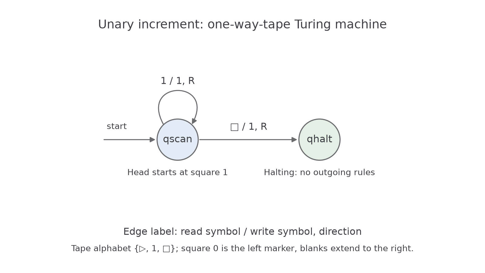
There is no outgoing rule from qhalt. These rules never move left and never read the marker from the stated start configuration. A diagram need not invent unreachable marker transitions. For unary input 11, the trace is:
| Completed steps | State | Head square | Tape squares 0–4 |
|---|---|---|---|
| 0 | qscan | 1 | ▷ 1 1 □ □ |
| 1 | qscan | 2 | ▷ 1 1 □ □ |
| 2 | qscan | 3 | ▷ 1 1 □ □ |
| 3 | qhalt | 4 | ▷ 1 1 1 □ |
The tape now represents three. The final head scans a blank at square 4, but it does not take another step because the state is halting. For input zero, the first scanned square is blank, so one step writes a 1 and halts. For n input 1 symbols, n scan steps and one final write give n + 1 steps. Keep a finite window in the trace while remembering that blanks continue indefinitely to the right.
To construct the diagram in a notebook, draw the start arrow, a qscan self-loop labelled 1 / 1, R, and an edge to qhalt labelled □ / 1, R. Halting is determined by having no outgoing transitions; an accepting-state double circle from FSM notation is not needed to mean “halt”.
A transition simulator
A simulator implements the formal transition rules as data and uses an algorithm to update the configuration.
Use strings > and _ for the marker and blank in Python, corresponding to ▷ and □ in the formal model. A dictionary maps tape positions to stored symbols; absent positions are blank. A second dictionary maps (state, read_symbol) to (new_state, write_symbol, direction). This representation lets the same simulator execute different rule tables. It is an implementation of the model, not its definition.
Continue this lesson.
You’re previewing NovaLearn without an account. Create a free account to read the rest.
Create free account