4.4.4.1–4.4.4.3 - Functions, growth and algorithm complexity (Python)
Use functions to describe how work grows with input size. Compare time and memory, calculate permutations and derive Big-O from an algorithm's actual operations rather than from the presence of a loop alone.
Functions and growth
A mathematical function maps each value in its domain to exactly one value in its co-domain.
Domain and co-domain
The domain is the set of permitted inputs. The co-domain is the declared set from which outputs are drawn. The range is the set of outputs actually produced and may be a smaller subset of the co-domain.
For example, , , maps each permitted natural number to one natural number. Here take . The co-domain is all natural numbers, while the range contains only even natural numbers. A mapping that assigns two different outputs to the same input is not a function. A Python function is a programming construct; it can implement a mathematical mapping, but the two ideas should not be confused.
The important complexity input is usually a size , such as the number of records, rather than a particular record's value. Four useful mathematical forms are:
| Form | Example | Effect of a size change |
|---|---|---|
| Linear | Doubling x doubles y | |
| Polynomial | Doubling x multiplies y by four | |
| Exponential | Increasing x by one doubles y | |
| Logarithmic | , for | Multiplying x by ten increases y by one |
[DIAGRAM: asset_slug: growth_functions; description: Exact plots of linear, quadratic, exponential and logarithmic functions with separate labelled axis scales]
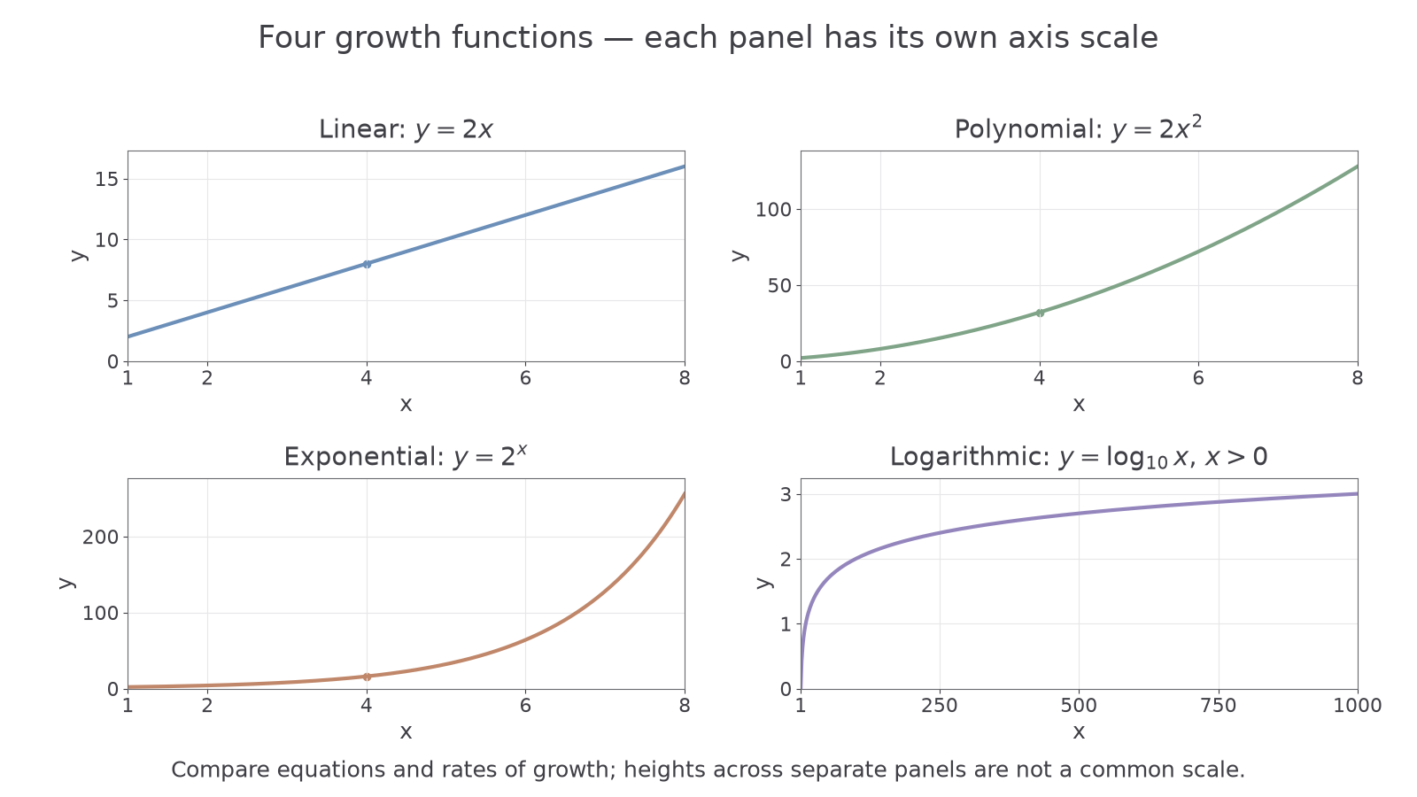
The panels use different vertical scales; compare their equations and rates of growth rather than the heights of different panels. For x = 4, the first three values are 8, 32 and 16. An exponential need not exceed a polynomial at every small input. Eventually exponential growth outpaces any fixed-degree polynomial.
Permutations and factorials
A permutation is an arrangement in which the order of the objects matters.
For three distinct letters A, B and C there are three choices for the first position, two remaining choices for the second and one for the last. Therefore there are arrangements: ABC, ACB, BAC, BCA, CAB and CBA. Choosing a group of letters without caring about order is a different problem.
The number of permutations of n distinct objects is
Also : there is one empty arrangement.
Four distinct objects have orders; five have . Going from n distinct objects to n + 1 multiplies the number of orders by n + 1. If an algorithm explicitly tries every order, the number of candidates is factorial. For ten distinct objects this is . Doubling the number of objects is therefore very different from doubling the work of a one-pass scan.
The distinct-object assumption is essential. The letters in ABA do not have six distinct visible arrangements: swapping its two identical A letters does not produce a new word. Do not apply the distinct-object count without checking the problem's assumptions. No repeated-object formula is needed here.
Time and space complexity
Algorithms can use different amounts of time and memory to solve the same-sized problem.
Time complexity describes how required operations grow with the size of the input. Counting operations avoids depending entirely on a particular computer, interpreter or momentary load. A timing measurement can be useful evidence, but a fast run on one small input does not establish a better growth rate.
Continue this lesson.
You’re previewing NovaLearn without an account. Create a free account to read the rest.
Create free account