Average speed from distance and time

Imagine timing a cyclist over a measured 200 m stretch. The cyclist may speed up and slow down within the stretch, so one distance and one total time tell us the average speed for the whole interval, not the speed at every instant.

Distance is measured in metres (m), time in seconds (s) and speed in metres per second (m/s). The words total distance and total time matter: when a journey has several stages, add all the distances and all the times before dividing.

Worked example: finding average speed

A train travels 1.35 km in 90 s. Convert the distance first:

$1.35 \mathrm{km} = 1.35 \times 1000 = 1350 \mathrm{m}$

Choose the relationship, substitute and calculate:

average speed = 1350 m / 90 s = 15 m/s

The answer is plausible because travelling at 15 m/s for 90 s gives $15 \times 90 = 1350 \mathrm{m}$, the stated distance.

The rearranged form finds distance directly. A cart moving at an average speed of 4.5 m/s for 32 s travels:

distance = 4.5 m/s × 32 s = 144 m

The units also check the method: $(m/s) \times s = m$.

Worked example: a journey with a wait. A walker covers 120 m in 80 s, waits 20 s, then covers 60 m in 40 s. The total distance is 180 m and the total time is 140 s, including the wait. The average speed is $180/140 = 1.29 \mathrm{m}/s$ (3 significant figures). Dividing by only the moving time answers a different question. Averaging the two stage speeds is generally unreliable because stages can last different times.

If speed is given in km/h, convert both units: $36 \mathrm{km}/h = 36 000 \mathrm{m} / 3600 \mathrm{s} = 10 \mathrm{m}/s$. Thus divide a km/h value by 3.6 to obtain m/s.

Reading distance-time graphs

A distance-time graph is a representation of how the accumulated distance travelled changes. Time is on the horizontal axis and distance is on the vertical axis. A point at (7 s, 8 m) means that after 7 s the object has travelled a total distance of 8 m; it does not show the object's route through space.

[DIAGRAM: asset_name: 03_1PH0-P1-02B_2.6-2.11 - Speed, acceleration and motion graphs - diagram 01; asset_slug: 1ph0-p1-02b-speed-acceleration-motion-graphs_diagram_01; recommended_method: matplotlib; description: Exact distance-time graph with labelled axes, three piecewise-linear journey stages, a horizontal rest interval, and a clearly constructed gradient triangle.]

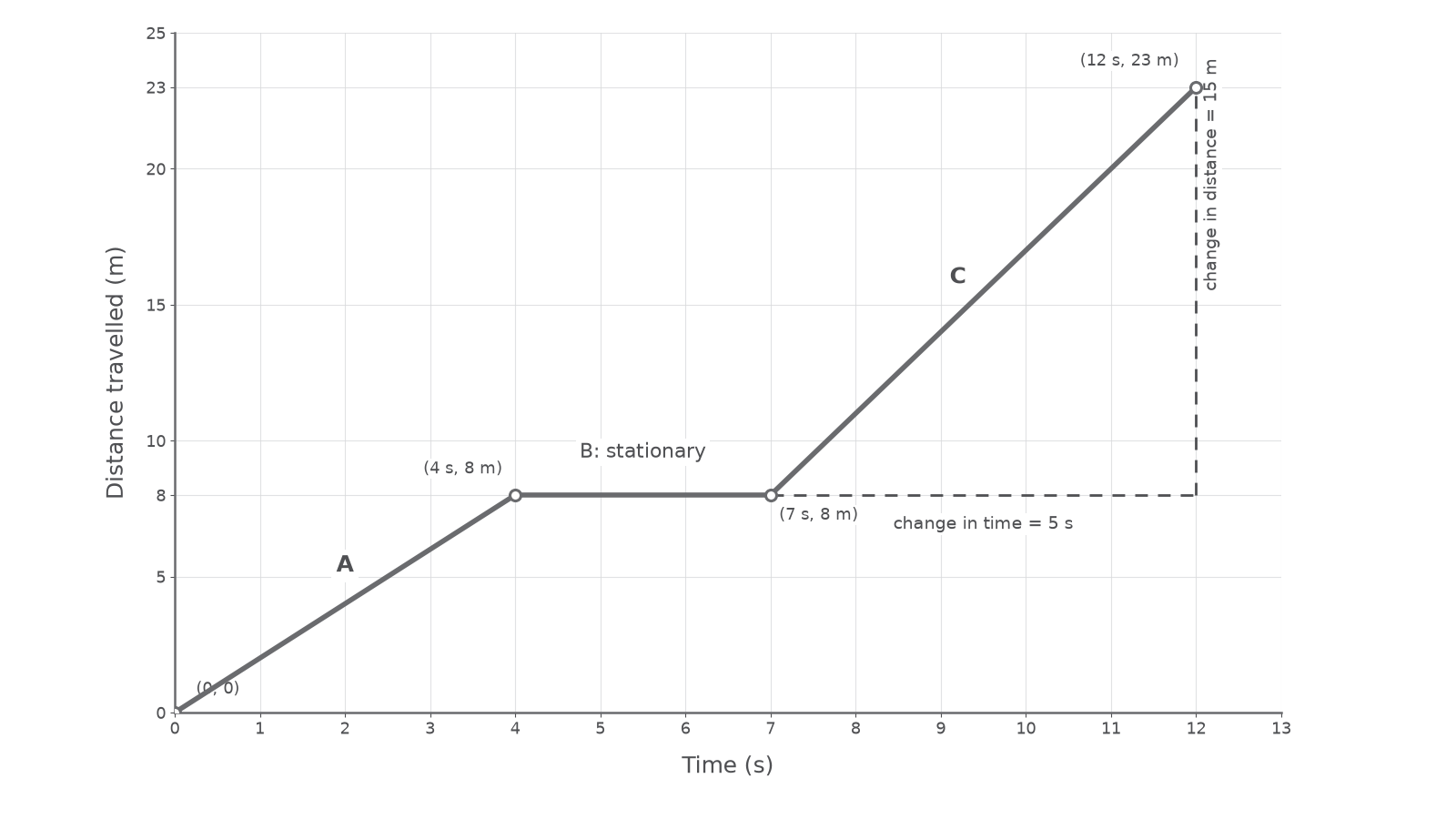
Read a distance-time graph in this order:

1. Check the axis quantities, units and scale.
2. Read the coordinates at the start and end of the interval of interest.
3. Describe what changes: an upward line means distance is increasing; a horizontal line means distance is unchanged, so the object is stationary.
4. Use the gradient to find speed.

For stage C in the graph, distance rises from 8 m at 7 s to 23 m at 12 s:

change in distance = 23 - 8 = 15 m

change in time = 12 - 7 = 5 s

speed = 15 m / 5 s = 3.0 m/s

A straight sloping line has constant gradient, so it shows constant speed. A steeper straight line has a larger gradient and therefore a greater speed. On a curved distance-time line, the gradient changes, so the speed changes; no tangent calculation is required in this lesson.

A graph of total distance travelled cannot slope down: distance accumulates. A graph labelled distance from the starting point can slope down when an object returns towards the start. Read the axis label before deciding what a downward segment means.