2.19 - Force, mass and acceleration core practical
Investigate why adding mass to a trolley changes its acceleration. Measure the driving force and motion, control the comparison, then use repeat readings and graphs to test the model and its limitations.
What the practical tests
Imagine releasing the same trolley twice, but adding a stack of masses before the second run. If the pulling force is kept constant, the heavier system should gain speed more slowly: it should have a smaller acceleration.
The aim is to investigate how the acceleration of a trolley changes when its mass is varied while the driving force is kept constant. The model being tested is Newton's second law.
resultant force = mass x acceleration
For a constant resultant force, . If the total accelerated mass doubles, the ideal model predicts that the acceleration halves.
Here, mass is a scalar measured in kilograms. Force and acceleration are vectors, but the trolley moves along one line, so the graph compares their magnitudes; the acceleration is along the resultant force. The measured relationship will be approximate because friction and measurement uncertainty cannot be removed completely.
Apparatus and variables
[DIAGRAM: asset_name: 05_1PH0-P1-02D_2.19 - Force, mass and acceleration core practical - diagram 01; asset_slug: 05_1ph0-p1-02d_2-19-force-mass-and-acceleration-core-practical_diagram_01; recommended_method: image_gen; description: A wide monochrome side-view apparatus diagram showing the inclined trolley ramp, added masses, two aligned light gates, pulley, fixed hanging mass and padded catch box.]
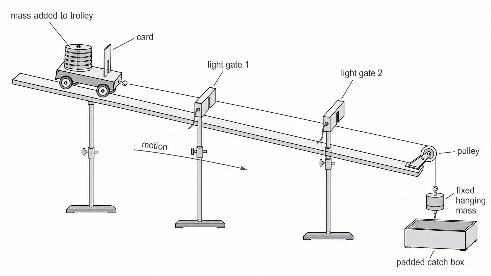
The apparatus consists of a dynamics trolley on a secured, slightly inclined ramp; a card fixed vertically to the trolley; two light gates connected to a datalogger; a pulley and string; a fixed hanging mass; slotted masses for the trolley; a balance; a suitable-range newton meter; and a padded catch box. The slight incline compensates for some wheel friction. It does not make friction exactly zero.
Choose the system before applying the model. The trolley, the masses on it and the fixed hanging mass all accelerate, so all belong to the total accelerated mass. The hanging mass's weight is an external driving force on this combined system. The string tension is internal to the combined system and should not simply be called equal to the hanging weight while the system accelerates.
| Variable role | Quantity | How it is handled |
|---|---|---|
| Independent | Total accelerated mass, in kg | Add measured masses to the trolley. Include the fixed hanging mass when comparing quantitatively with . |
| Dependent | Acceleration, in m/s | Calculate it from two light-gate velocities and the time between them, then find a mean. |
| Controlled | Driving force | Keep the hanging mass unchanged for every run. |
| Controlled | Release and measurement conditions | Use the same trolley, ramp slope, start mark, card, light-gate positions, string and pulley. |
The diagram omits the datalogger connected to the gate leads. Record measured driving force in N, total accelerated mass in kg and timing readings in s. After approximate friction compensation, the measured hanging weight estimates the net external force on the combined trolley–hanger system. Residual friction, the slope component of weight and pulley resistance limit that approximation; a constant hanger alone does not prove that the net force is exactly constant.
Method and measurements
- Secure the ramp and pulley. Adjust the small slope so that it approximately compensates for the trolley's wheel friction, then mark one release position.
- Measure the mass of the trolley, each added mass and the fixed hanging mass with a balance. Measure the card length with a millimetre ruler and enter it into the datalogger.
- Before assembling the moving system, zero the newton meter, suspend the hanger and its fixed load, wait until stationary, and record their weight in newtons. Cross-check with the measured hanger mass using . This measures the external gravitational driving force on the combined system; it is not a measurement of the string tension during acceleration. Then attach the trolley to the fixed hanging mass with a taut string over the pulley. Place a padded catch box below the hanger and make the string short enough that the trolley cannot strike the pulley.
- Position light gate 1 near the start and light gate 2 farther down the ramp. Check that the card passes centrally through both gates without touching them.
- Check that the hanger will remain in free motion until both velocity readings and the intervening time are recorded. If it lands in the catch box earlier, the driving force changes and the run is invalid. Release the trolley from the mark without pushing it. The logger uses card length divided by the interruption time at each gate to obtain the first velocity and second velocity . It also records the time between those velocity readings. Use the logger’s paired-velocity timing mode; for long cards, the interval should match the midpoints of the two interruption measurements rather than mismatched leading/trailing edges.
- Return the trolley to the same mark and repeat the run twice more. Three readings at one mass reveal random variation and allow a mean acceleration to be calculated.
- Add a measured mass securely to the trolley and repeat steps 5-6. Use at least five well-spaced total masses while keeping the hanging mass and all other controls unchanged.
The genuine hazards are moving equipment and falling masses. Keep feet and fingers away from the hanger, use the padded catch box, secure the ramp and pulley, and stop the trolley before it reaches the end. Goggles are not a substitute for controlling these mechanical hazards.
Process and graph the data
For each run, calculate acceleration from the change in velocity and the time over which that change occurs.
and are velocities in m/s, is time in s, and is acceleration in m/s.
Worked example. For one run with a total accelerated mass of 0.70 kg, the logger records , and .
The acceleration is positive because the trolley's velocity increases in the chosen positive direction. A gain of 0.43 m/s in half a second makes 0.86 m/s a plausible result.
The following original results show three repeats and a mean for each mass.
| Total accelerated mass, (kg) | Run 1 (m/s) | Run 2 (m/s) | Run 3 (m/s) | Mean (m/s) |
|---|---|---|---|---|
| 0.50 | 1.15 | 1.18 | 1.17 | 1.17 |
| 0.60 | 0.96 | 1.01 | 1.00 | 0.99 |
| 0.70 | 0.84 | 0.88 | 0.86 | 0.86 |
| 0.80 | 0.73 | 0.75 | 0.74 | 0.74 |
| 1.00 | 0.58 | 0.61 | 0.58 | 0.59 |
[DIAGRAM: asset_name: 05_1PH0-P1-02D_2.19 - Force, mass and acceleration core practical - diagram 02; asset_slug: 05_1ph0-p1-02d_2-19-force-mass-and-acceleration-core-practical_diagram_02; recommended_method: matplotlib; description: Two exact quantitative graphs plot the original lesson data as acceleration against mass and acceleration against reciprocal mass, with labelled axes, units and fitted relationships.]
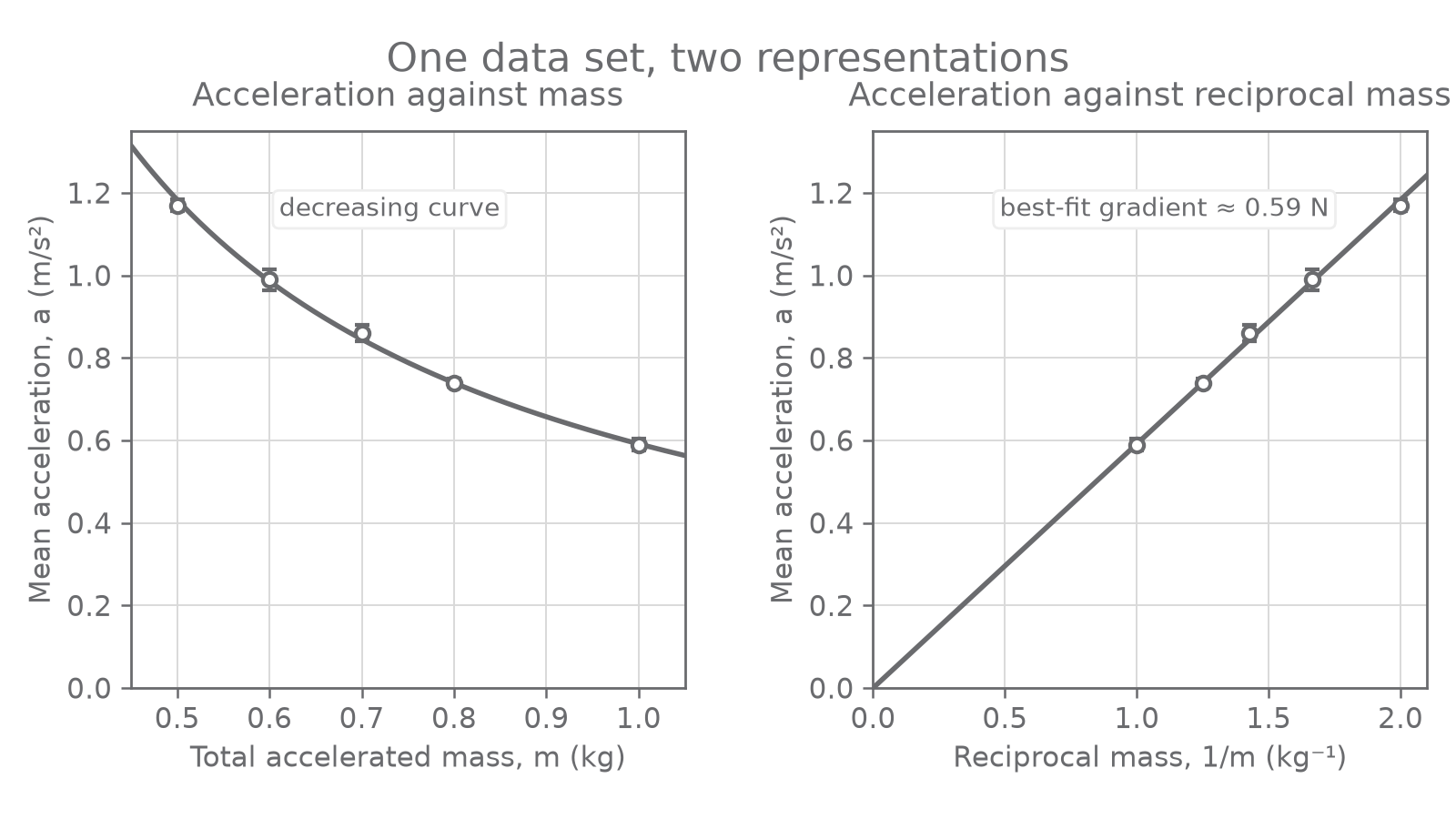
On the left graph, the horizontal axis is total accelerated mass and the vertical axis is mean acceleration. The points follow a decreasing curve, not a straight line. On the right, the same acceleration values are plotted against ; the near-straight best-fit line shows that is approximately proportional to . A best-fit relationship represents the trend, so the points should not be joined dot to dot.
Evaluate the evidence
The data support the prediction: when the driving force is constant, increasing total mass decreases acceleration. The reciprocal-mass graph is close to a straight line, so the evidence supports . It does not prove that the apparatus is ideal.
Use the spread of repeats to judge repeatability. For example, the three accelerations at 0.60 kg have a range of . A result far from the other repeats should be checked and repeated; it should not be deleted merely because it is inconvenient. Taking a mean reduces the effect of random variation, but it does not remove systematic error.
| Limitation | Specific improvement | Why it helps |
|---|---|---|
| A hand release can give the trolley a small extra push. | Hold the trolley against a fixed stop at the start mark and use a mechanical release that moves clear without pushing. | Each run begins from the same position without an additional force, improving validity and repeatability. |
| Residual wheel or pulley friction changes the resultant force. | Adjust the ramp until the unloaded trolley moves at nearly constant velocity after a gentle push, and keep the same trolley and pulley for all runs. | A constant velocity indicates a resultant force close to zero before the hanger is attached, reducing systematic bias from friction. |
| An incorrect card length biases both light-gate velocities. | Measure the card along its direction of travel, view the ruler square-on, check the ruler zero and independently check the value entered into the logger. | Square-on measurement reduces parallax; checking the zero and entered value addresses systematic errors that a mean alone cannot remove. |
Light gates make the timing automatic and avoid human reaction time, but their alignment and the entered card length still matter. A push that ends before both gates need not change the later acceleration in an ideal constant-force model. A push-free release still keeps initial conditions comparable and avoids lingering hand contact.
A strong conclusion therefore combines the expected graph shape, small repeat ranges and a method that keeps the force and release conditions controlled.
Check friction compensation with representative added masses as well as the unloaded trolley while keeping the chosen ramp slope fixed. If loaded trolleys clearly speed up or slow down before the hanger is attached, report that the constant-net-force approximation is poor; improve the apparatus before collecting the final series. Repeating readings cannot correct this systematic problem.
As a force check, calculate m × mean acceleration. The example data give values close to 0.59 N (for 0.50 kg: ). Compare this with the measured hanger weight, allowing for residual forces and uncertainty. On the reciprocal-mass graph the gradient has units , so it estimates the net force. The small vertical bars show the spread of repeated accelerations about their mean; they are not extra data points.