1.1.4 - Price elasticity of supply
Learn how to calculate and interpret producers’ responsiveness to price, draw different supply responses and explain why manufacturing and primary production often respond differently.
Calculating PES
Producers can respond to a higher selling price only if they can make more output available.
Price elasticity of supply (PES) measures the responsiveness of quantity supplied to a change in the good’s own price, holding other influences on supply constant. It describes movement along a supply curve rather than a shift caused by a cost or technology change.
Price elasticity of supply
For an ordinary upward-sloping supply curve, price and quantity supplied change in the same direction, so PES is positive. Illustrative data: the price of containers rises from £4 to £5, and weekly quantity supplied rises from 800 to 1,000. Price rises ; quantity rises . PES = 25 ÷ 25 = 1. It has no currency or percent unit.
If price falls 10% and quantity supplied falls 5%, PES = −5 ÷ −10 = 0.5, also positive. Use the original value as the percentage base unless another convention is explicitly specified. When percentages are given, divide those percentages directly. Quantity supplied means what producers are willing and able to offer at each price, not necessarily what customers eventually buy.
Supply values and diagrams
The size of PES shows whether the percentage output response is smaller than, equal to or greater than the price change.
| PES | Classification | Interpretation |
|---|---|---|
| 0 | Perfectly price inelastic | No quantity response; vertical supply. |
| Above 0, below 1 | Price inelastic | Smaller percentage quantity response. |
| 1 | Unitary price elastic | Equal percentage quantity and price changes. |
| Above 1 | Price elastic | Larger percentage quantity response. |
| Limiting infinity | Perfectly price elastic | Additional output is available at a fixed price in the idealised model; horizontal supply. |
Use common axes with price vertically and quantity horizontally. The illustrative schedules below all pass through A: price £5, quantity 100 units per week. Plot the points and draw straight supply lines S₁, S₂ and S₃.
| Price (£) | S₁ quantity | S₂ quantity | S₃ quantity |
|---|---|---|---|
| 4 | 60 | 90 | 80 |
| 5 | 100 | 100 | 100 |
| 6 | 140 | 110 | 120 |
From A to £6, price rises 20%. S₁ quantity rises 40%, so PES = 2; S₂ rises 10%, so PES = 0.5; S₃ rises 20%, so PES = 1. At the common reference point and on these common scales, the flatter line has the larger response. Slope alone is not elasticity: the initial price and quantity determine the percentage comparison.
The straight unit-elastic supply line passes through the origin. Along S₃, quantity is 20 times price, so an equal proportional price change always produces an equal proportional quantity change. A straight supply line does not automatically have PES = 1. Compare S₁’s positive price-axis intercept with S₂’s positive quantity-axis intercept; neither passes through the origin.
[DIAGRAM: asset_name: Supply elasticity at a common point; asset_slug: 4ec1_e10_supply; caption: Unit-elastic straight supply passes through the origin; description: Same-scale supply lines with elastic, inelastic and unitary responses at price 5 quantity 100, plus separate vertical and horizontal limiting curves.]
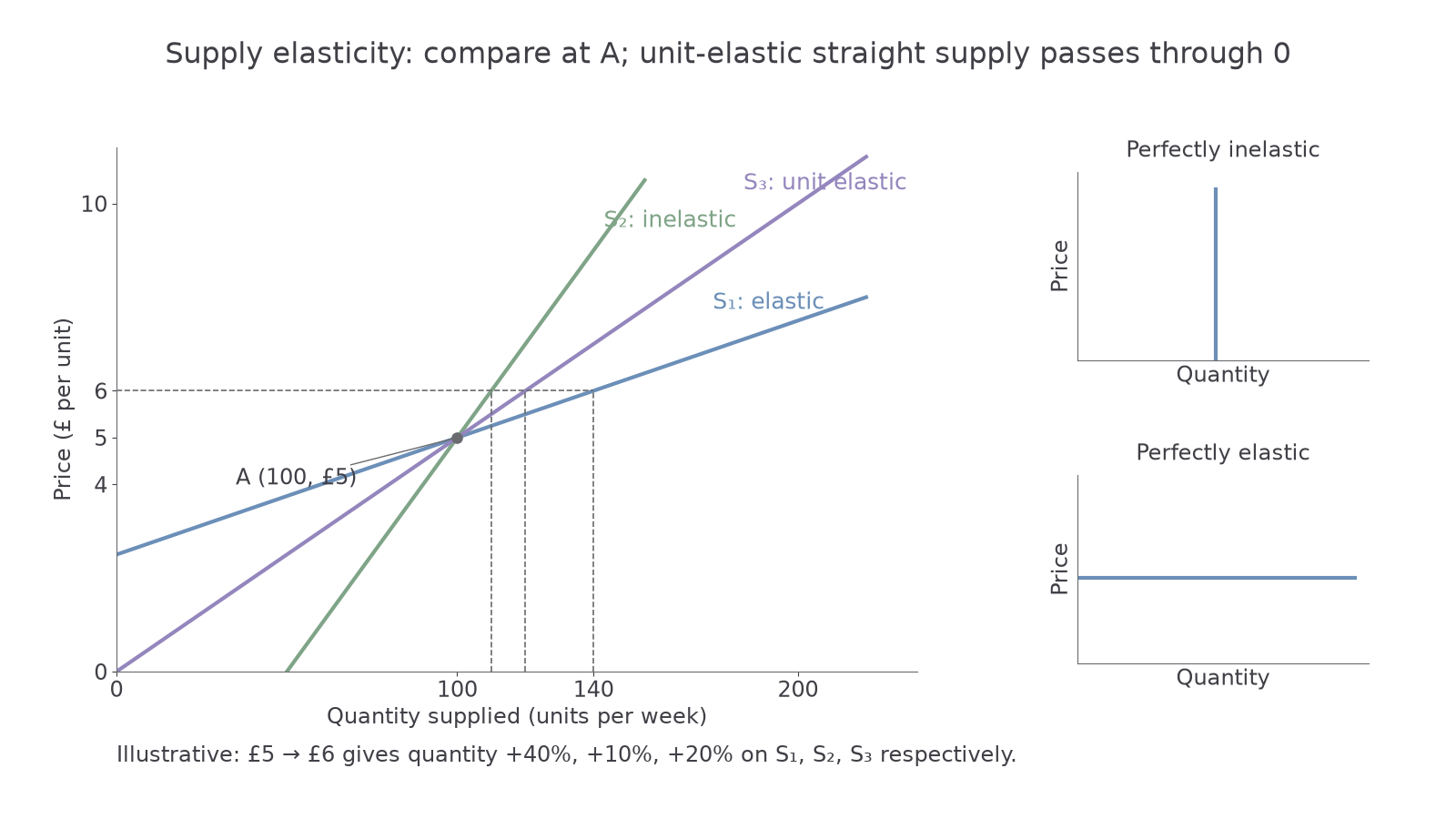
Optional notebook construction — ungraded: plot the three schedules, label axes and A, extend S₃ to the origin, and sketch vertical and horizontal supply separately. Check the changes from £5 to £6 against the table. Text interpretation can be scored in the app; your actual drawing is not submitted or marked here.
Capacity, resources and stocks
The practical ability to expand output determines how strongly quantity supplied responds to a higher price.
Factors of production must be available and usable. A furniture producer may need suitable timber, skilled workers and machinery. If these resources are readily available, it can expand production. If skilled workers are scarce or a specialised machine takes months to obtain, the response is restricted. Mobility matters too: a worker who can move between tasks makes expansion easier than one whose skills apply only to an unrelated activity.
Spare capacity means unused productive resources within a firm. A factory running one shift may add another or use idle machines when prices rise. A factory already operating at full capacity cannot do this easily, so its short-run PES is likely lower. Spare capacity must actually be usable: idle machines without staff do not guarantee an output response.
Availability of stocks allows firms to increase the quantity offered without waiting for new production. A wholesaler holding canned food can release stock quickly. Fresh fish or ripe berries cannot usually be held for long, limiting this adjustment. Stocks are finite: once they are exhausted, continued expansion requires more production. Storage can also be expensive, so stocks do not always exist even for non-perishable goods.
Time and product comparisons
Supply usually becomes more responsive when producers have longer to obtain resources and adjust capacity.
In the very short run, output may already be fixed. Over weeks, a firm can use stocks, add overtime and hire workers. Over years, it can build facilities and develop new production methods. Therefore time often raises PES, although scarce land, regulations or difficult technology can continue to limit expansion.
Manufactured products are made by transforming materials. Standard notebooks can often be produced using additional shifts, stored and supplied from existing inventories. Their PES may be relatively high if materials and machines are available. A specialised aircraft is also manufactured, but skilled labour, safety requirements and long production times may make its supply inelastic in the short run. “Manufactured” is not itself a guarantee of elastic supply.
Primary products are obtained from natural resources, such as farming, fishing and mining. A coffee grower cannot instantly mature new plants when prices rise. Weather, land and the growing cycle restrict short-run output; fresh produce also has limited storage. These conditions tend to make primary supply inelastic. Yet stored grain can be released quickly, and over several seasons farmers can change acreage, so the comparison depends on the product and period.
Compare an illustrative stationery factory with a strawberry farm after a price rise lasting one week. The factory with spare machines and stored materials can respond immediately; the farm’s harvest depends on plants already grown. Over several years, both can invest, making the contrast smaller. Explain the production constraint rather than merely repeating the category label.