1.1.4 - Measuring price elasticity of demand
Learn how to measure consumers’ responsiveness to price, interpret the signed result and construct demand curves that show different degrees of responsiveness.
Measuring responsiveness
A price rise can cause a very small or a very large fall in purchases; price elasticity measures the size of that response.
Price elasticity of demand (PED) is the responsiveness of quantity demanded to a change in the good’s own price, with other influences on demand held constant. It concerns movement along a demand curve. A change in income or fashion shifts demand and must not be mistaken for the response to price alone.
Price elasticity of demand
Using percentages makes comparisons possible between products measured in different units. A reduction of 100 cinema tickets says little without knowing whether initial sales were 200 or 20,000. Elasticity has no currency, quantity or percent unit: the two percentages divide out.
For an ordinary downward-sloping demand curve, price and quantity demanded move in opposite directions. A 5% price rise and a 15% quantity fall give PED = −15 ÷ 5 = −3. Retain the negative sign in the calculation. The magnitude, here 3, determines whether the response is elastic or inelastic. Some reports quote only the magnitude; write clearly which convention you are using.
Percentage bases and calculation
The original value is the base when a question asks for the percentage change from an initial price or quantity.
Illustrative data: a bicycle rental raises its hourly price from £10 to £12. Weekly hours rented fall from 500 to 350. The price change is . The quantity change is . PED is −30 ÷ 20 = −1.5. Purchases fall proportionately more than price rises.
If percentage changes are already supplied, divide them directly; do not divide the quantity percentage by the new price in pounds. If quantity falls, its percentage change is negative. A price fall is also negative, so a quantity rise divided by a price fall again gives negative PED. For example, +12% ÷ −6% = −2.
Use the base specified in the question. A midpoint convention averages the initial and final values, but it is a different calculation; do not switch conventions partway through. Estimates using original bases describe the stated interval. They need not be identical for a reverse change using a different base. Round the final result to the requested precision, keeping unrounded working beforehand.
Interpreting PED values
Classification compares the size of the percentage quantity response with the size of the percentage price change.
| Signed PED | Classification | Meaning |
|---|---|---|
| 0 | Perfectly price inelastic | Quantity does not respond to price. |
| Between −1 and 0 | Price inelastic | Quantity changes by a smaller percentage than price. |
| −1 | Unitary price elastic | Quantity and price change by equal percentages in opposite directions. |
| Below −1, such as −2 | Price elastic | Quantity changes by a larger percentage than price. |
| Limiting magnitude of infinity | Perfectly price elastic | Buyers will buy at the given market price, but none at a higher price in the idealised model. |
Thus −0.4 is inelastic and −2.5 is elastic. “More negative” does not mean “less responsive”: −2.5 has the larger magnitude. Unitary elasticity is the dividing case, not perfectly elastic demand. A perfectly elastic curve is horizontal; a perfectly inelastic curve is vertical. These are useful limiting models rather than a claim that every real product has an extreme response.
For unitary elasticity at every point, a curved demand relationship with constant price × quantity can be drawn. A straight downward-sloping curve is unit elastic only at a particular point, not throughout.
Constructing and reading demand curves
A demand diagram must identify price vertically and quantity horizontally, and comparisons must use common scales and a common reference point.
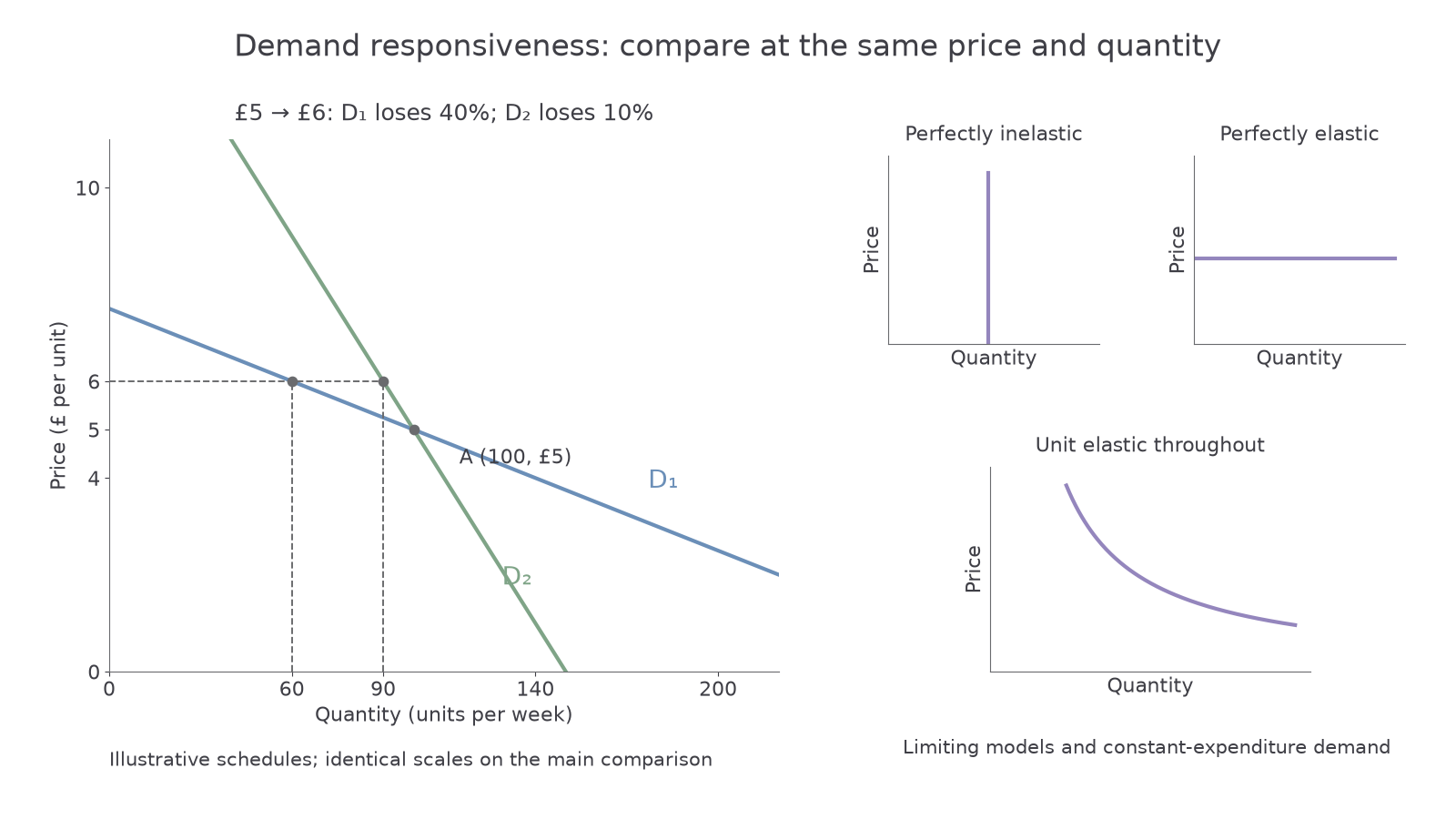
The illustrative schedules below share price £5 and quantity 100. Plot each schedule on the same axes, with quantity in units per week and price in pounds per unit. Mark the common point A, then join each set of points with its own labelled straight curve.
| Price (£) | Quantity on D₁ | Quantity on D₂ |
|---|---|---|
| 4 | 140 | 110 |
| 5 | 100 | 100 |
| 6 | 60 | 90 |
From A to a price of £6, price rises 20%. D₁ quantity falls 40%, giving PED −2; D₂ quantity falls 10%, giving PED −0.5. D₁ is more responsive over this change. On these same scales and at A, D₁ is flatter and more elastic. Slope alone is not elasticity: stretching an axis changes the apparent slope without changing the economic percentages. Curves compared at different prices and quantities can also mislead.
[DIAGRAM: asset_name: Demand responsiveness at a common point; asset_slug: 4ec1_e08_responsiveness; caption: Common scales and point A allow a valid comparison of the two demand responses; description: Two demand schedules through price 5 quantity 100, with separate small panels showing vertical, horizontal and constant-expenditure demand.]
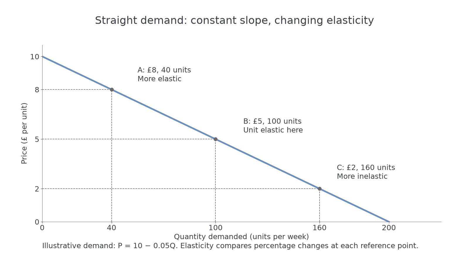
The second graph uses the single straight line . Around its high-price, low-quantity point (£8, 40), a £1 rise cuts quantity by 20: quantity falls 50%, price rises 12.5%, giving PED −4. Around its low-price, high-quantity point (£2, 160), the same £1 rise cuts quantity by 20: −12.5% ÷ 50% = −0.25. The slope is unchanged, yet elasticity changes. At the middle point (£5, 100), a small change gives PED −1. This is why the entire straight line cannot simply be labelled “elastic”.
[DIAGRAM: asset_name: Elasticity along straight demand; asset_slug: 4ec1_e08_varying; caption: The same straight demand curve has elastic and inelastic regions; description: Demand line from price 10 quantity 0 to price 0 quantity 200 with labelled high, middle and low points.]
Optional notebook construction — ungraded: reproduce the schedules on labelled axes, identify A and the two new quantities at £6, and sketch the vertical and horizontal limiting curves on separate axes. Self-check units, scales, labels and whether the price rise produces a movement along each curve. The app’s text answers can check interpretation; they do not assess your actual drawing.