1.1.3 - Market equilibrium and changing markets
Combine demand and supply to find market equilibrium, construct it from data, and explain how shifts alter price and quantity in everyday market situations.
Finding and drawing equilibrium
Market equilibrium occurs at the price where the quantity consumers wish to buy equals the quantity producers offer for sale.
At the equilibrium price, quantity demanded equals quantity supplied. Their common value is the equilibrium quantity. Neither curve determines the market result alone: buyers may prefer a lower price, while sellers may prefer a higher one. The intersection identifies a price–quantity combination compatible with both plans. It does not mean that every person can afford the good or that the outcome is socially desirable.
This illustrative weekly fruit-box market has the following schedules:
| Price per box | Quantity demanded | Quantity supplied |
|---|---|---|
| £2 | 100 | 20 |
| £4 | 80 | 40 |
| £6 | 60 | 60 |
| £8 | 40 | 80 |
| £10 | 20 | 100 |
The £6 row shows equality at 60 boxes per week. To construct the equilibrium, label price (£ per box) vertically and quantity (boxes per week) horizontally. Choose regular scales. Plot each demand and supply pair with quantity first, joining the demand points as D1 and supply points as S1. Mark their intersection E1 and draw horizontal and vertical guide lines to read £6 and 60. These guides are readings, not new curves. The original curves appear in both diagrams below.
Away from £6, the schedules disagree; that creates pressure for price adjustment, examined in the next lesson. Here, equilibrium means that there is no excess demand or supply at the stated price. Keep all conditions fixed when describing a particular equilibrium.
Optional notebook construction — ungraded. Draw D1 and S1 from the five rows, then label E1, £6 and 60 boxes per week. Self-check the two opposite slopes, intersection and axis guides against an original E1 in the supplied diagrams. This paper task practises drawing; the app's text input does not assess official Draw performance.
Demand shifts and market outcomes
A demand shift changes the equilibrium even when producers' supply relationship stays unchanged.
Suppose a successful campaign makes fruit boxes more popular. At each price consumers now want 40 more boxes per week. Demand shifts right from D1 to D2. The new intersection with unchanged S1 is E2: price rises from £6 to £8 and equilibrium quantity from 60 to 80. Producers extend quantity supplied along S1 as the selling price rises; supply has not shifted. The rightward demand shift is the cause, while the higher price and quantity are the resulting market outcome.
A fall in popularity reverses the direction. If demand shifts left to D0, the new intersection E0 is £4 and 40 boxes. Lower demand therefore reduces equilibrium price and quantity, other conditions unchanged, and quantity supplied contracts along S1.
[DIAGRAM: asset_name: Demand shifts and equilibrium; asset_slug: 4ec1_e06_demand_shift; caption: With supply unchanged, increased demand raises equilibrium price and quantity; decreased demand lowers both.; description: Two fruit-box panels show original E1 at 60 and £6; demand increase gives E2 at 80 and £8, while demand decrease gives E0 at 40 and £4.]
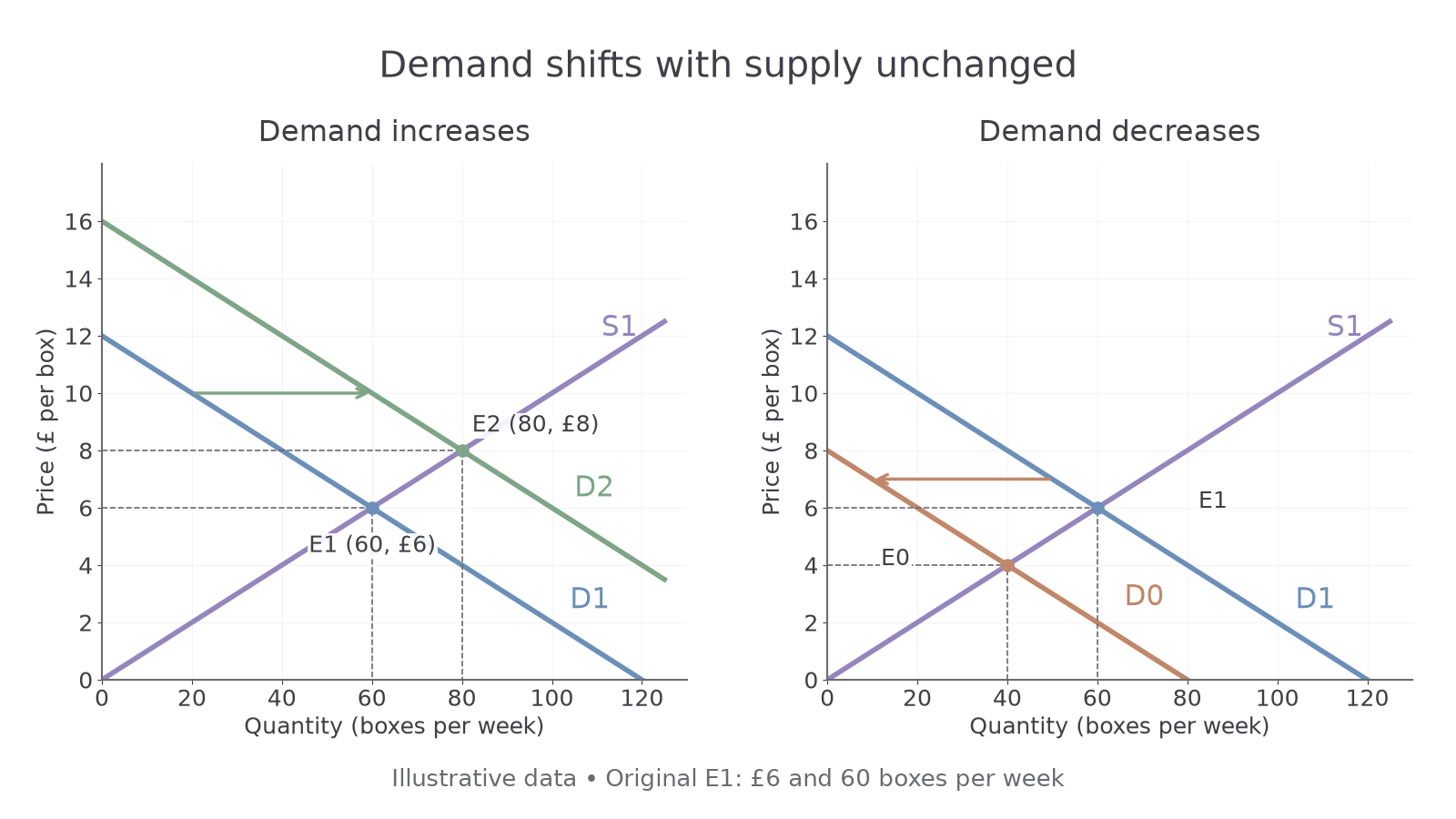
To construct either change, preserve the original D1 and S1 and mark E1. Add the new demand curve, labelled D2 or D0, to the correct side. Mark its new intersection with S1 and project to both axes. A shift arrow runs between demand curves; the new equilibrium is not found by keeping the old price or quantity fixed. The increased-demand schedule is 40 boxes above original demand at each listed price; decreased demand is 40 below where the quantity remains non-negative.
For an illustrative everyday application, more commuters moving into a town could increase demand for local rail travel. With the same supply relationship, equilibrium fares and journeys rise. The diagram predicts direction under its assumptions; actual fares may be controlled and fixed capacity may limit the quantity response. Specify those conditions rather than treating every observed price change as proof of one demand cause.
Supply shifts and market outcomes
A supply shift changes price and quantity in opposite directions when demand is unchanged.
Suppose improved sorting equipment reduces the cost of preparing fruit boxes. Suppliers offer 40 more boxes at each price, shifting supply right from S1 to S2. At the new intersection with unchanged D1, E2, price falls from £6 to £4 while quantity rises from 60 to 80. Buyers extend quantity demanded along D1 because the fruit's own price is lower. Demand has not shifted: its relationship with price remains the same.
If drought reduces the available fruit harvest, supply can instead shift left to S0. In the illustrative diagram E0 is at £8 and 40 boxes. The reduced supply raises equilibrium price and lowers equilibrium quantity, while quantity demanded contracts along the unchanged demand curve. A poor harvest does not, by itself, make consumers want less fruit at each price.
[DIAGRAM: asset_name: Supply shifts and equilibrium; asset_slug: 4ec1_e06_supply_shift; caption: With demand unchanged, increased supply lowers price and raises quantity; decreased supply raises price and lowers quantity.; description: Two fruit-box panels show original E1 at 60 and £6; supply increase gives E2 at 80 and £4, while supply decrease gives E0 at 40 and £8.]
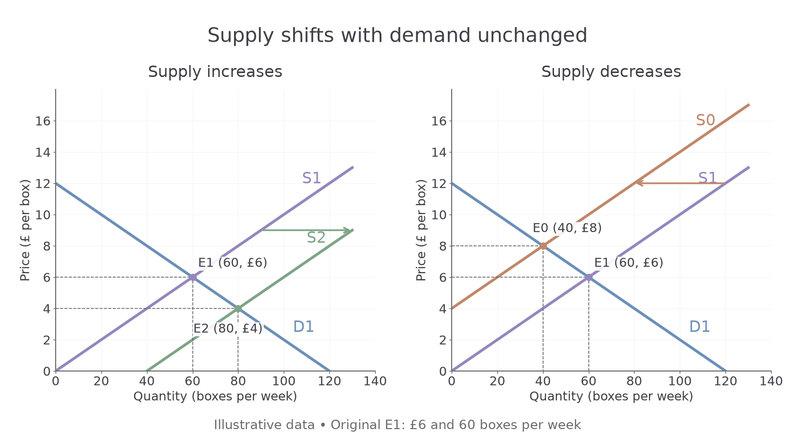
For construction, retain D1 and S1, add the new supply curve and mark its intersection with D1. Use a rightward shift arrow for S2 or a leftward one for S0, then read the new guides to both axes. The increased-supply schedule is 40 boxes above original supply at each listed price; the decreased schedule is 40 below where output stays non-negative.
These mechanisms matter in actual types of markets: better refrigeration can reduce the cost and loss involved in supplying food; a storm can interrupt fish landings. Each situation requires identifying its effect on producers before predicting the price–quantity result. Price falls do not prove that demand fell: an increase in supply also lowers price, but it raises quantity instead.
Using directions and conditions
A reliable prediction starts by identifying which underlying relationship changes and what is held constant.
For a single shift, the results can be organised as follows:
| Change, other curve unchanged | Equilibrium price | Equilibrium quantity |
|---|---|---|
| Demand increases | Rises | Rises |
| Demand decreases | Falls | Falls |
| Supply increases | Falls | Rises |
| Supply decreases | Rises | Falls |
The table records consequences, but the causal explanation remains essential. A lower input cost changes suppliers' willingness to produce at every selling price; it is not a demand change. A rise in a substitute's price changes buyers' willingness at every own price; it is not a supply change. Move only the curve justified by the case, and distinguish its shift from the movement along the other curve.
Sometimes both curves shift. If an advertising campaign raises fruit demand while improved sorting raises supply, both changes tend to increase equilibrium quantity. Their price effects oppose one another: demand pushes price up and supply pushes it down. The final price can rise, fall or remain unchanged depending on the relative size of the shifts. With demand rising and supply falling, price rises, but quantity is ambiguous. Do not invent a precise result when the case provides no information to settle these opposing effects.
Direction is also different from magnitude. Two rightward demand shifts of different sizes need not produce equal price rises. A graph with actual schedules can give numerical equilibria; a diagram without numeric scales usually supports directional reasoning only. The model holds other relevant conditions constant and assumes market price is able to adjust.