1.1.1 - Production possibility curves and growth
Use a production possibility curve to show productive limits, resource use and opportunity cost, then distinguish a change in output from a change in an economy's productive capacity.
Constructing a production frontier
A production possibility curve shows the maximum combinations of two outputs an economy can produce with its available resources and technology.
The production possibility curve (PPC) is also called the production possibility frontier (PPF). To simplify the whole economy, put all output into two categories. The illustrative economy below divides its resources between food and machinery. Both quantities are measured per year. Each row is a maximum combination: obtaining more machinery requires releasing resources from food production.
| Machinery (units per year) | Food (tonnes per year) |
|---|---|
| 0 | 100 |
| 20 | 96 |
| 40 | 84 |
| 60 | 64 |
| 80 | 36 |
| 100 | 0 |
Start a graph at the origin. Label the horizontal axis “Machinery (units per year)” and the vertical axis “Food (tonnes per year)”. Choose equal, regular intervals along each individual axis: here intervals of 20 fit both scales. Plot machinery first, then food: the third row is the point (40, 84), not (84, 40). Join the frontier points with a smooth downward-sloping curve labelled PPF. Do not join each point to the origin. The curve is a simplified model between the observed combinations.
[DIAGRAM: asset_name: Productive limits and resource use; asset_slug: 4ec1_e02_frontier; caption: The frontier joins maximum output combinations; U is inside and V is outside the current productive limit.; description: Illustrative food and machinery PPF with A at 40 and 84, B at 60 and 64, U at 40 and 50 and V at 60 and 90.]
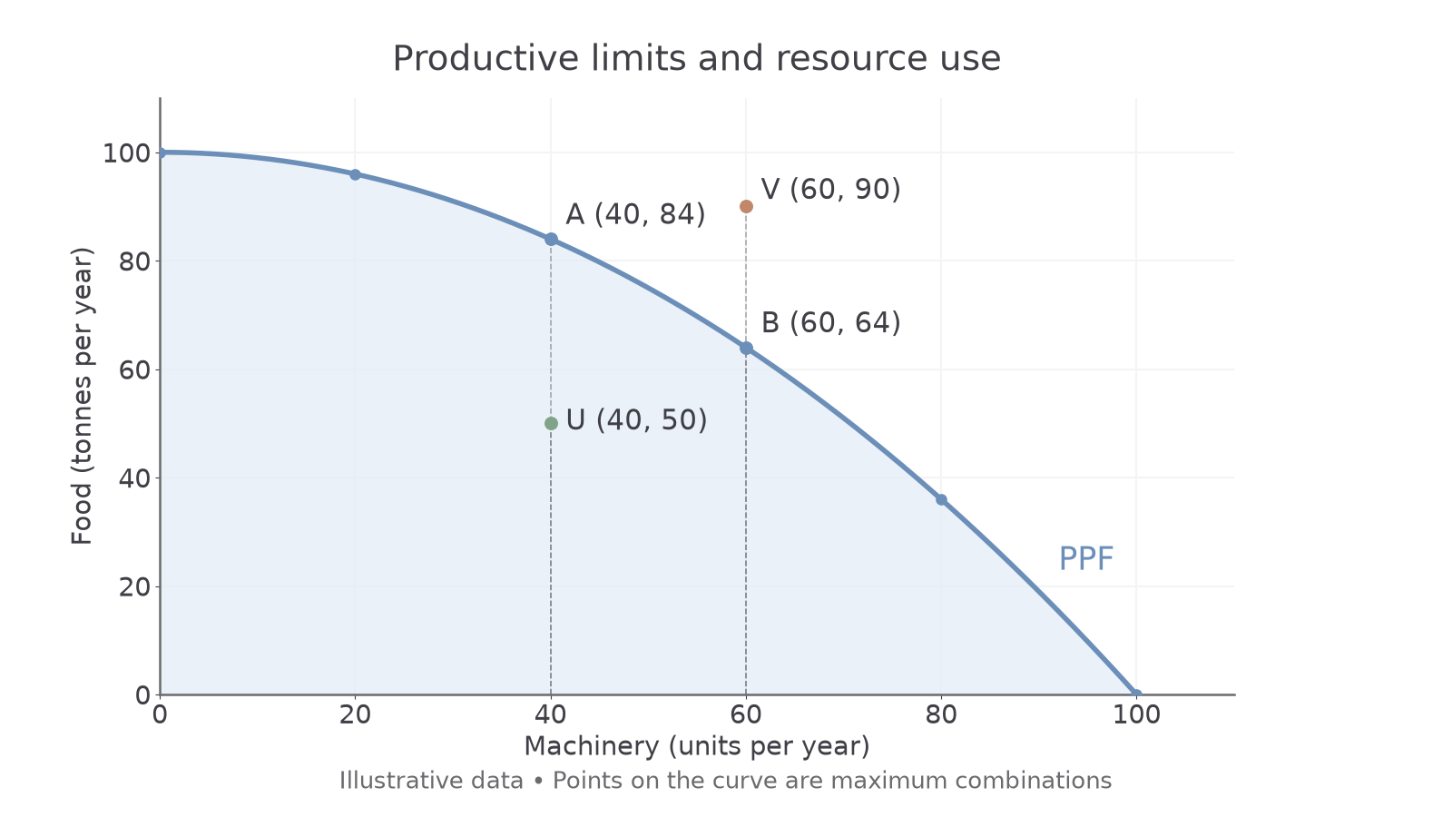
Optional notebook construction — ungraded. Plot the table yourself and add A at (40, 84), U at (40, 50) and V at (60, 90). Self-check the labelled axes, regular scales, correct coordinates and curve through all six frontier points against the supplied graph. This develops actual drawing skill; the app's text questions do not grade a submitted drawing.
Possible output and resource use
A point's position relative to the frontier tells us whether it is attainable and whether the available productive resources are being fully used.
Points on the frontier, such as A and B, represent the maximum productive potential for that output mix. Resources are fully employed and used efficiently within this model. More food cannot be produced there without giving up some machinery. This does not prove that the chosen mix best meets society's wants: the model shows what can be produced, not what ought to be produced.
A point inside the frontier, such as U, is possible but below maximum potential. Some resources may be unemployed, such as workers without jobs or idle equipment. Resources might also be used inefficiently. At U the economy produces 40 machines and 50 tonnes of food, although A shows that 84 tonnes are possible with the same machinery output. Bringing unused resources into production could increase food without sacrificing machinery. A movement from U towards the existing frontier is greater actual output, not an outward shift of capacity.
A point outside the frontier, such as V, is unobtainable with current resources and technology. At 60 machines the present maximum food output is 64 tonnes, so 90 tonnes is beyond the limit. It could become attainable after productive capacity increases. “Unobtainable” therefore means under the stated current conditions, not forever.
Opportunity cost on the frontier
Moving along a frontier makes the sacrifice required for additional output visible.
From A to B, machinery rises from 40 to 60 units while food falls from 84 to 64 tonnes. The opportunity cost of those 20 extra machines is the 20 tonnes of food forgone. Per additional machine over this interval, the cost is one tonne of food. Use the change in the sacrificed output, rather than the remaining food output of 64 tonnes.
Farther along this curved frontier, moving from 80 to 100 machines sacrifices 36 tonnes of food for 20 machines: 1.8 tonnes per extra machine. The frontier bows out from the origin because resources are not equally suited to every use. As machinery production expands, increasingly suitable food-producing resources have to be transferred, raising the food sacrificed. A straight frontier would instead represent a constant opportunity cost. Both are simplified models; the curve does not mean money is being paid for each transfer.
The downward slope expresses scarcity. When productive resources are already fully and efficiently employed, producing more of one good requires producing less of another. A point inside the curve is different: using idle resources can raise both outputs before this frontier trade-off is reached.
Capacity growth and contraction
The whole frontier shifts when an economy's productive potential changes.
An outward shift means positive growth in productive capacity: more combinations become attainable. More workers, investment in additional equipment and infrastructure, improved skills, or better technology can raise the quantity or effectiveness of resources. For example, reliable electricity can reduce equipment downtime, allowing the same workforce to produce more. If an improvement benefits only machinery production, that axis's maximum may rise more than the food maximum; shifts need not be parallel.
An inward shift means a loss of productive capacity. A natural disaster can destroy factories and farmland; war can damage infrastructure or reduce the available workforce; long-term deterioration of equipment can also lower potential output. In the illustrative diagram, the maximum on each axis falls from 100 to 80 after a capacity loss, or rises to 120 after a capacity gain.
[DIAGRAM: asset_name: Expanding and contracting capacity; asset_slug: 4ec1_e02_growth; caption: PPF1 is the original limit; PPF2 shows more productive capacity and PPF0 shows less.; description: Three illustrative PPF curves with maxima of 80, 100 and 120 on food and machinery axes, with outward and inward shift arrows.]
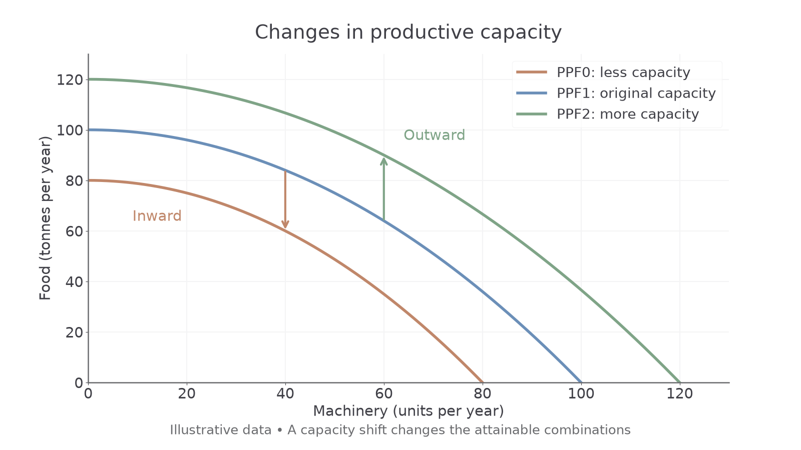
Growth of actual output and growth of potential output must be distinguished. An economy can produce more by employing previously idle resources, moving towards an unchanged PPF. Conversely, a demand-led fall in actual production can move it inside an unchanged frontier. A recession alone does not prove that resources or technology have deteriorated. This lesson uses frontier shifts to represent positive or negative changes in productive potential; a later lesson measures actual economic growth using GDP.
Greater potential also does not guarantee full use of it. Newly trained workers can remain unemployed. To explain a shift, name the resource or productivity change that alters the maximum attainable combinations, then distinguish it from changing utilisation of existing capacity.