Drag as a fluid force

Drag is a contact force. It happens because an object moving through a fluid must push fluid particles out of the way and energy is transferred to the surroundings.

In this specification, a fluid means a liquid or a gas. Air is a fluid, so air resistance is one example of drag. Oil, water and glycerol are also fluids, so a ball bearing falling through a viscous liquid experiences drag too.

The direction matters. If an object falls vertically downwards through still air, drag acts upwards. If an object moves horizontally to the right through air, drag acts to the left. If the air itself is moving, what matters is the object's motion relative to the air.

For an object travelling through air, the drag is affected by factors such as:

• speed of the object through the air
• cross-sectional area facing the motion
• shape and streamlining
• surface texture
• air density

The most important pattern for this lesson is that, for the same object in the same fluid, drag increases as speed increases. The exact formula is not a recall equation here. If a question wants you to use a particular drag relationship, it will be given in the question.

Falling with changing acceleration

A falling object in a uniform gravitational field has an approximately constant weight $W = mg$. Drag is different: it depends on the motion through the fluid, so it changes as the speed changes.

For a falling object in air where upthrust is negligible:

Here $W$ is the weight in newtons and $D$ is the drag in newtons. The positive direction in this expression is taken as downwards.

[DIAGRAM: asset_name: Lesson 3.02.2: Drag and terminal velocity - diagram 01; asset_slug: 3_02_2_drag_and_terminal_velocity__diagram_01; recommended_method: drawn_physics; description: Three-panel force diagram for a sphere falling through air: at release v = 0, weight downward and negligible drag; while speeding up, same weight downward and smaller upward drag so resultant is downward; at terminal velocity, upward drag equals downward weight and resultant is zero. Use thin grey arrows and labels W = mg, D, resultant.]

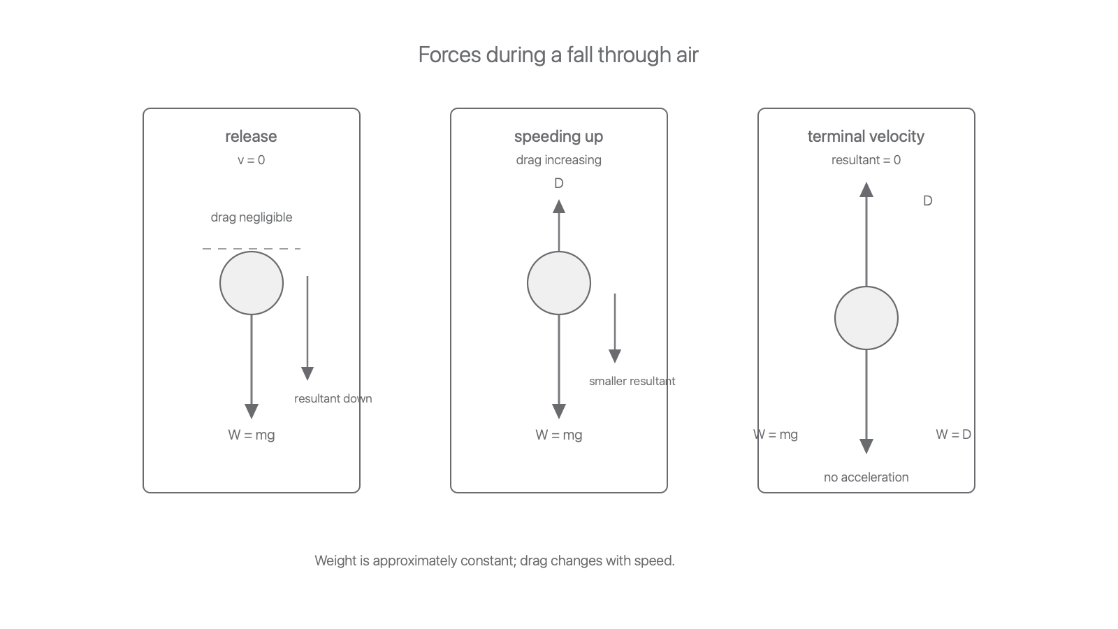
At the instant of release, the object's speed is zero, so drag is usually negligible. The resultant force is almost equal to the weight, so the initial acceleration is close to $g$ if upthrust is negligible.

As the object speeds up, drag increases. The downward resultant force becomes smaller:

so the downward acceleration also becomes smaller. This is non-uniform acceleration because the acceleration is not constant.

[DIAGRAM: asset_name: Lesson 3.02.2: Drag and terminal velocity - diagram 02; asset_slug: 3_02_2_drag_and_terminal_velocity__diagram_02; recommended_method: drawn_physics; description: Velocity-time graph for an object falling from rest with drag. Curve rises steeply then levels towards a dashed horizontal line labelled terminal velocity. Add two tangents/gradient labels showing acceleration decreases as gradient decreases. Axes labelled time / s and velocity / m s^-1.]

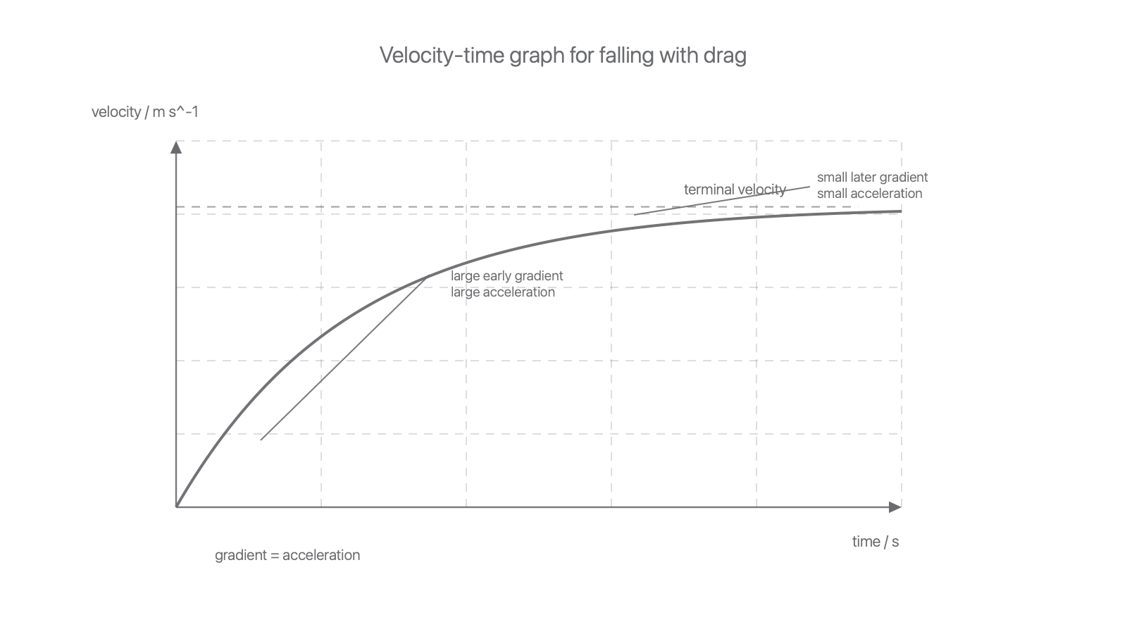
On a velocity-time graph, the gradient is acceleration. For falling with drag, the graph is steep at first, then gradually becomes less steep as drag increases. When the graph becomes horizontal, the gradient is zero and the acceleration is zero.

Worked example: finding drag from a graph

A ball of mass $1.8 \times 10^{-2}\,\text{kg}$ falls through air. At one instant, a tangent to its velocity-time graph gives an acceleration of $2.1\,\text{m s}^{-2}$ downwards. Upthrust is negligible. Calculate the drag at this instant.

First calculate the weight:

Use $F_{\text{resultant}} = ma$:

The resultant force is downwards, so:

To two significant figures, the drag is:

The answer is less than the weight, which makes sense because the object is still accelerating downwards.

Terminal velocity

Terminal velocity is reached when the forces on the falling object have adjusted so that the resultant force is zero. The object is still moving, but it is no longer accelerating.

For a falling object in air, where upthrust is negligible, terminal velocity occurs when:

In a liquid, upthrust may not be negligible. Then the vertical terminal balance is:

where $U$ is the upthrust.

This is a common trap: terminal velocity does not mean there are no forces. It means the downward and upward forces balance, so the resultant force is zero. Newton's second law then gives $a = 0$, so the velocity is constant.

Now compare two falling objects with the same shape and size but different masses. At the same speed, their drag is about the same because the speed, shape and cross-sectional area are the same. The heavier object has a larger weight, so at that same speed it has a larger downward resultant force. It must speed up more before drag becomes large enough to balance its weight. Therefore it has a larger terminal velocity.

Worked reasoning: hollow ball and sand-filled ball

A hollow plastic ball and the same ball partly filled with sand are dropped through air. At $0.50\,\text{m s}^{-1}$, the drag on them is the same because their shape, size and speed are the same. The sand-filled ball has a larger weight, so its downward resultant force is larger at this speed.

The sand-filled ball reaches terminal velocity only when drag has increased enough to balance this larger weight. Since drag increases with speed, that happens at a greater speed. So the sand-filled ball has the greater terminal velocity.

Determining terminal velocity

OCR links this topic to PAG1-style techniques for determining terminal velocity in fluids. Two common approaches are a ball bearing falling through a viscous liquid and paper cones falling through air.

[DIAGRAM: asset_name: Lesson 3.02.2: Drag and terminal velocity - diagram 03; asset_slug: 3_02_2_drag_and_terminal_velocity__diagram_03; recommended_method: drawn_physics; description: Apparatus layout for determining terminal velocity of a ball bearing in viscous liquid: tall transparent tube or measuring cylinder filled with viscous liquid, ball bearing falling, release point, upper and lower timing marks separated by distance s, ruler beside tube, stopwatch/light gate/video camera, and note that timing marks are below the acceleration region.]

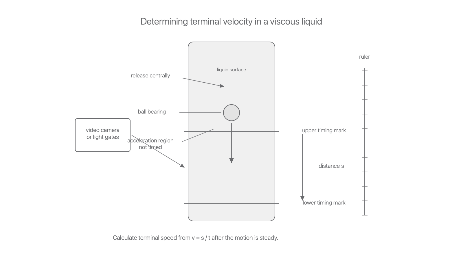
For a ball bearing in a viscous liquid, a good method is:

1. Fill a tall transparent tube with viscous liquid and mark two horizontal timing lines a known distance $s$ apart.
2. Place the first timing mark far enough below the surface for the ball bearing to have reached terminal velocity before timing begins.
3. Release the ball bearing gently from rest at the centre of the tube, avoiding sideways motion and bubbles.
4. Measure the time $t$ for the ball to travel between the two timing marks, using light gates, video analysis or a stopwatch.
5. Calculate the terminal velocity using $v = s/t$, then repeat and calculate a mean.
6. If investigating a factor affecting terminal velocity, change one independent variable and keep the key control variables constant.

For paper cones in air, the same principle applies: measure the time for a cone, or stack of cones, to pass through a known distance after it has settled into steady motion. A motion sensor, light gates or video analysis can reduce reaction-time uncertainty.

In a terminal-velocity investigation, likely variables are:

• independent variable: for example number of nested cones, cone mass, ball radius, liquid type or temperature
• dependent variable: terminal velocity
• control variables: shape and cross-sectional area where appropriate, release height, timing distance, fluid temperature, same tube/liquid, same ball material if radius is not being investigated

Good evaluation points include:

• Use a larger distance between timing marks to reduce percentage uncertainty in distance and time.
• Use video or light gates instead of manual timing to reduce reaction-time error.
• Repeat readings and identify anomalies before calculating a mean.
• Keep the liquid temperature constant because viscosity changes with temperature.
• Use a wide tube so wall effects do not significantly alter the motion of a ball bearing.
• Start timing only after the object has reached terminal velocity; one check is that equal distances lower down take equal times.

Worked example: calculating terminal velocity and uncertainty

A ball bearing travels between two timing marks separated by $0.300 \pm 0.001\,\text{m}$. The measured times are $0.94\,\text{s}$, $0.98\,\text{s}$ and $0.96\,\text{s}$.

The mean time is:

The terminal velocity is:

To three significant figures:

The spread in the time readings is $0.98 - 0.94 = 0.04\,\text{s}$, so a simple estimate of the uncertainty in the mean time is about $\pm 0.02\,\text{s}$.

Percentage uncertainty in distance:

Percentage uncertainty in time:

For $v = s/t$, combine the percentage uncertainties by adding them:

The absolute uncertainty in $v$ is approximately:

So a sensible result is:

This also tells you where the experiment needs improvement: timing contributes much more uncertainty than the measured distance.

Exam Patterns

Questions on this topic often combine ideas rather than asking for a single definition. You may be asked to:

• explain a force balance in words
• use a tangent to a velocity-time graph to find acceleration
• calculate resultant force using $F = ma$
• infer drag from $W - D = ma$
• explain why terminal velocity changes when mass, shape or fluid changes
• describe and evaluate a terminal-velocity practical
• interpret a supplied formula or proportionality for a sphere falling through a fluid

The safest reasoning chain for a falling object is:

1. Weight is approximately constant.
2. Drag acts opposite the motion and increases as speed increases.
3. Resultant force decreases as drag increases.
4. Acceleration decreases because $F_{\text{resultant}} = ma$.
5. At terminal velocity, resultant force is zero.

If a question gives you a formula for terminal velocity, treat it like any other supplied relationship. Identify which variables are being changed, hold the other variables constant, and state the proportionality carefully. For example, if a supplied expression shows $v \propto r^2$, then halving the radius would make terminal velocity one quarter as large, provided all other quantities in the expression are unchanged.

Exam Patterns Summary