Motion experiments turn a moving object into measurements: distances, times, speeds and accelerations. In this lesson you will compare common laboratory techniques for investigating motion, then use two practical routes to determine the acceleration of free fall, $g$ . The physics is familiar, but the marks usually come from matching the apparatus to the quantity measured and evaluating the quality of the data.

Motion apparatus and data

An investigation of motion needs a way to measure position or distance and a way to measure time. Different apparatus gives different kinds of data, so the best choice depends on the motion being studied.

Apparatus or technique	What it can measure or show	Typical strength	Typical limitation
Trolley and runway	position, distance and timing over a track	simple repeatable motion	friction and runway alignment matter
Air-track glider	near-frictionless straight-line motion	useful for motion and collision investigations	needs careful levelling and air supply
Ticker timer	dots at regular time intervals on tape	visual record of changing speed	tape drag and dot reading uncertainty
Light gates	time for a card or object to block a beam	small timing uncertainty	gives average speed over a finite length
Data logger	repeated electronic readings from sensors	many readings with consistent timing	sensor calibration and setup matter
Video analysis	position at successive frames	useful when motion is visible but hard to instrument	scale, parallax and frame rate limit accuracy

For motion and collision experiments, light gates or video can measure speeds before and after an interaction. A card of known length passing through a light gate gives:

Speed from a light gate

v \approx \frac{\text{length blocking the beam}}{\text{beam-block time}}

The symbol $\approx$ is important. The value is an average speed while the beam is blocked, not an exact instantaneous speed. The shorter the card or diameter, and the smaller the timing uncertainty, the closer the value is to the speed at that position.

When planning, name the variables clearly. The independent variable is the quantity deliberately changed, the dependent variable is the quantity measured as the outcome, and control variables are kept the same to make the test valid. For example, in a trolley experiment down a runway, the slope could be the independent variable, acceleration the dependent variable, and trolley mass/runway surface/release method control variables.

Free fall and g

Free fall has a precise meaning: the only significant force on the object is its weight. Near the Earth's surface, an object in free fall has a downward acceleration with magnitude about $9.81\ \text{m s}^{-2}$ .

Acceleration of free fall

The acceleration of free fall, $g$ , is the acceleration of an object when the only significant force acting on it is gravity. Near the Earth's surface, $g \approx 9.81\ \text{m s}^{-2}$ .

In a school laboratory, free fall is an ideal model. A dense steel ball dropped through a short distance is a reasonable approximation because air resistance is small compared with its weight. An inflated balloon is not a good approximation: air resistance is large compared with its weight, so the measured acceleration would be much smaller than $g$ .

The acceleration $g$ is independent of the falling object's mass when air resistance is negligible. A heavier object has a larger weight, but it also has more mass to accelerate. These effects balance in the ideal model, so mass alone does not make one object have a larger free-fall acceleration.

For a dropped object released from rest, the applied analysis often uses:

Drop from rest

h = \frac{1}{2}gt^2

Here $h$ is the vertical distance fallen in metres and $t$ is the time in seconds. This is the constant-acceleration equation $s = ut + \frac{1}{2}at^2$ with $u = 0$ , $s = h$ , and $a = g$ , using downward as positive.

Electromagnet and trapdoor method

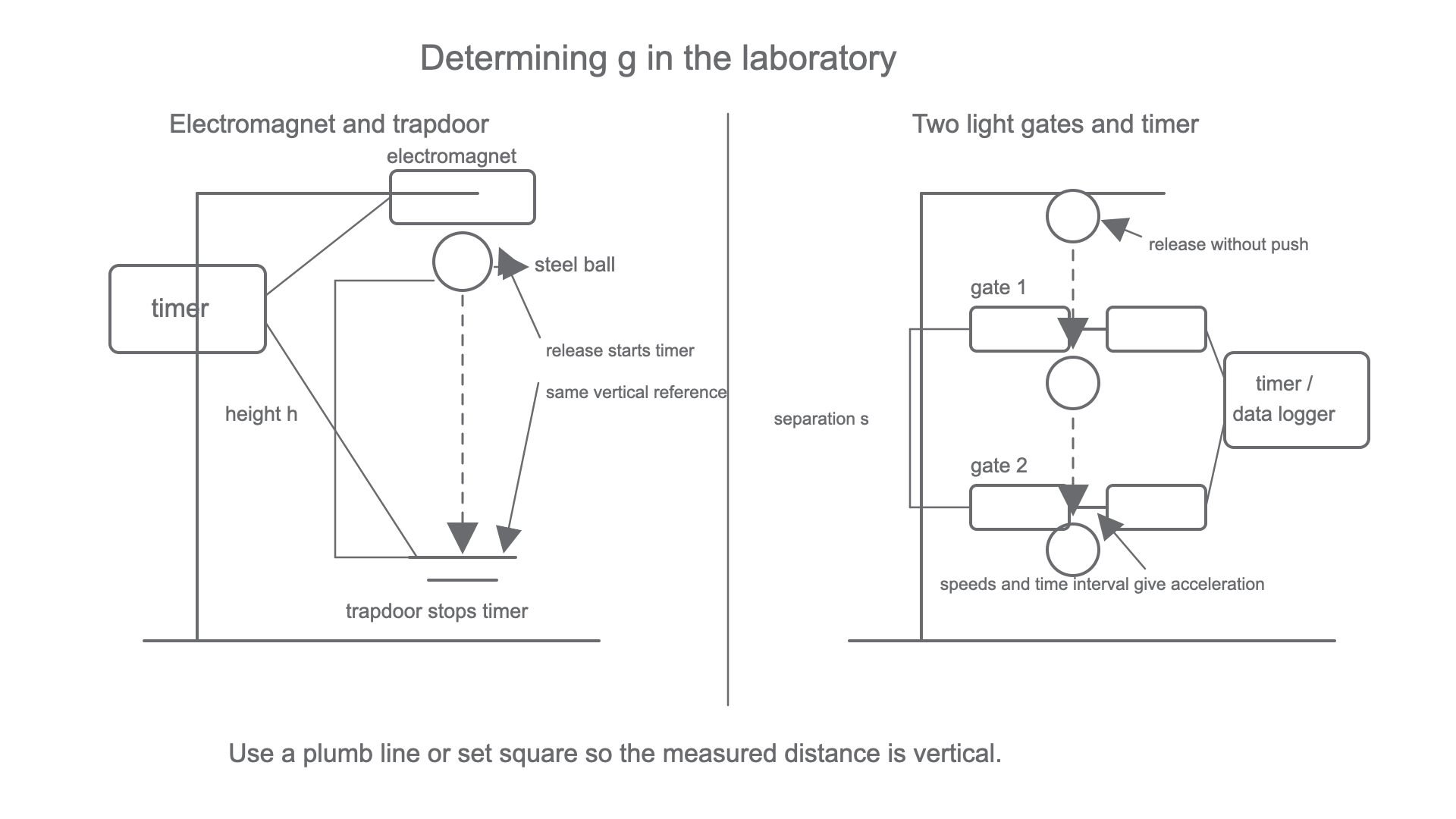
One method for determining $g$ releases a steel ball using an electromagnet. The same switching action starts the timer. When the ball reaches the trapdoor switch below, the timer stops.

[DIAGRAM: asset_name: Lesson 3.01.2b: Investigating Motion and Free Fall - diagram 01; asset_slug: 3_01_2b_investigating_motion_and_free_fall__diagram_01; recommended_method: drawn_physics; description: A clean 16:9 apparatus diagram comparing two laboratory routes to determine g. Left panel shows an electromagnet holding a steel ball above a trapdoor switch connected to a timer, with vertical height h, release starts timer, trapdoor stops timer, and consistent vertical reference. Right panel shows a falling ball through two light gates connected to a timer/data logger, labelled gate 1, gate 2, separation s, release without push, and speeds plus time interval give acceleration. White background, #6A6B6E only.]
Diagram

A method that can produce useful data is:

Hold a steel ball at the electromagnet and place the trapdoor directly below.
Measure the vertical distance $h$ from the release point to the point that triggers the stop signal. Use a plumb line or set square to keep this distance vertical.
Release the ball without pushing it, so the initial velocity is as close to zero as possible.
Record the time $t$ for the fall.
Repeat at the same height to identify anomalies and calculate a mean time.
Repeat for several different heights and process the data using a graph.

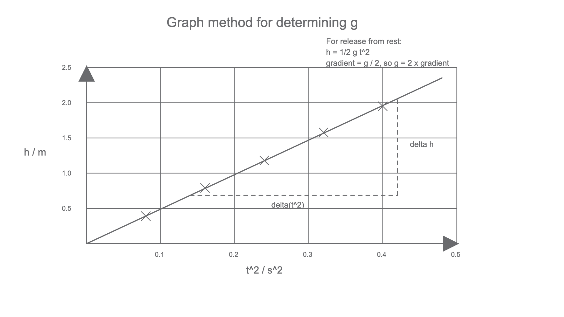
The graph route is stronger than relying on one drop. From:

h = \frac{1}{2}gt^2

a graph of $h$ on the vertical axis against $t^2$ on the horizontal axis should be a straight line through the origin. Its gradient is:

\text{gradient} = \frac{h}{t^2} = \frac{g}{2}

so:

Determining g from a graph

g = 2 \times \text{gradient of the } h \text{ against } t^2 \text{ graph}

[DIAGRAM: asset_name: Lesson 3.01.2b: Investigating Motion and Free Fall - diagram 03; asset_slug: 3_01_2b_investigating_motion_and_free_fall__diagram_03; recommended_method: drawn_physics; description: A clean 16:9 graph for determining g. Vertical axis h / m from 0 to 2.5, horizontal axis t^2 / s^2 from 0 to 0.5. Show plotted cross data close to a straight best-fit line through the origin, a dashed gradient triangle labelled delta h and delta(t^2), and text h = 1/2 g t^2; gradient = g/2; g = 2 x gradient. White background, #6A6B6E only.]
Diagram

Worked example: using a single drop as a first estimate

A steel ball is released from rest and falls through $1.20\ \text{m}$ . Three measured times are $0.497\ \text{s}$ , $0.492\ \text{s}$ and $0.495\ \text{s}$ .

Mean time:

\bar{t} = \frac{0.497 + 0.492 + 0.495}{3} = 0.4947\ \text{s}

For a first estimate:

h = \frac{1}{2}gt^2

so:

g = \frac{2h}{t^2}

Substitute:

g = \frac{2(1.20)}{(0.4947)^2} = 9.81\ \text{m s}^{-2}

This agrees very closely with the accepted value, but a graph from several heights would be more reliable because it uses more data and reduces the effect of one poorly timed drop.

Light gates and timers

Light gates can be used in two related ways. A single gate can find the speed of a falling object as it passes the gate. Two gates can find speeds at two positions and the time between those positions.

[DIAGRAM: asset_name: Lesson 3.01.2b: Investigating Motion and Free Fall - diagram 02; asset_slug: 3_01_2b_investigating_motion_and_free_fall__diagram_02; recommended_method: drawn_physics; description: A clean 16:9 diagram showing a falling object interrupting a light gate. Include the object diameter d across the beam, a downward motion path, and a timer signal trace with a rectangular dip from t1 to t2 labelled beam-block time = delta t. Include formula text v approx d / delta t and note that the value is average speed over the object's diameter. White background, #6A6B6E only.]
Diagram

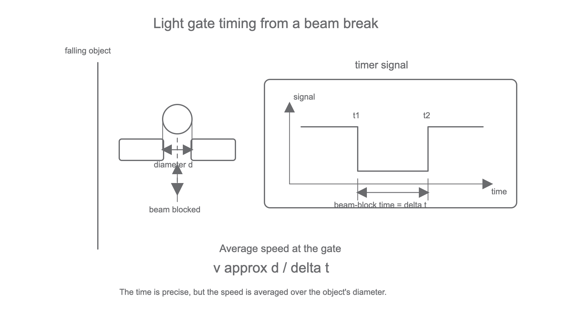
For one light gate:

v \approx \frac{d}{\Delta t}

where $d$ is the diameter of the ball or the length of the card blocking the beam, and $\Delta t$ is the beam-block time. If a ball is falling, the speed is increasing during the block interval, so this is an average speed near the gate.

For two light gates:

Measure the separation $s$ between the gates using a consistent vertical reference point.
Use the gate times to determine the speed $u$ at the first gate and $v$ at the second gate.
Use the timer or data logger to measure the time interval $t$ between the two speed measurements.
Determine the acceleration using:

Acceleration from two gate speeds

a = \frac{v-u}{t}

If air resistance is negligible and the object was falling freely between the gates, this acceleration is an experimental value for $g$ .

Worked example: two light gates

A ball of diameter $16.0\ \text{mm}$ falls through two light gates. At gate 1, the beam-block time is $7.60\ \text{ms}$ . At gate 2, the beam-block time is $5.00\ \text{ms}$ . The time between the two speed measurements is $0.110\ \text{s}$ .

Convert the diameter and times:

d = 16.0\ \text{mm} = 0.0160\ \text{m}

7.60\ \text{ms} = 7.60 \times 10^{-3}\ \text{s}

5.00\ \text{ms} = 5.00 \times 10^{-3}\ \text{s}

Speed at gate 1:

u \approx \frac{0.0160}{7.60 \times 10^{-3}} = 2.11\ \text{m s}^{-1}

Speed at gate 2:

v \approx \frac{0.0160}{5.00 \times 10^{-3}} = 3.20\ \text{m s}^{-1}

Acceleration between the gates, using the unrounded speed values:

a = \frac{v-u}{t} = \frac{\frac{0.0160}{5.00 \times 10^{-3}}-\frac{0.0160}{7.60 \times 10^{-3}}}{0.110} = 9.95\ \text{m s}^{-2}

This is close to $9.81\ \text{m s}^{-2}$ , so the data are consistent with free fall within normal laboratory uncertainty.

Uncertainty, errors and improvements

Determining $g$ is not complete when a number appears on the calculator. A good practical answer also discusses how trustworthy the number is.

Important sources of uncertainty and error include:

distance measurement: parallax, measuring from inconsistent points, or a drop path that is not vertical
timing: human response time for stopwatch methods, trigger delay, or finite beam-block length in light-gate methods
release method: pushing the object accidentally gives a non-zero initial velocity
air resistance: drag reduces the measured acceleration, especially for light or large-area objects
alignment: the object may miss the gate centre, clip the trapdoor unevenly, or move sideways

Useful improvements follow directly from these limitations. Use a dense small object, release it without a push, align the drop vertically with a plumb line, use electronic timing, repeat readings, use several heights, plot a best-fit line, and use a large gradient triangle rather than two nearby plotted points.

Safety is simple but still real: secure clamps and stands, use a catcher or tray for falling balls, keep feet and hands away from the impact region, and avoid placing fragile sensors where the object can strike them.

When comparing an experimental value with an accepted value, use percentage difference:

Percentage difference

\text{percentage difference} = \frac{|\text{experimental value} - \text{accepted value}|}{\text{accepted value}} \times 100\%

Small percentage difference suggests good accuracy, but it does not prove the method is valid by itself. Two systematic errors can sometimes cancel. Always connect the numerical comparison to the method.

Last Accessed

Module 1

Development of practical skills in physics

Foundations of physics

Module 3

Forces and motion

Electrons, waves and photons

Module 5

Newtonian world and astrophysics

Module 6

Particles and medical physics

3.1.2(a)(ii),(b) - Motion and free-fall investigations