1.2.2(k)-(l) - ICT, data logging and ionising radiation
This lesson is about using modern practical tools well: data loggers, sensors, software, computer models and radiation detectors. These can be assessed as practical techniques, so the skill is not just naming equipment. You need to explain why a tool is suitable, how to set it up, how to process the data, and how to work safely with ionising radiation and draw a justified conclusion.
Digital Tools in Practical Physics
Outcome 1.2.2(k) covers three closely linked ideas: computer modelling, data logging with sensors, and software processing of data. They all use ICT, but they do different jobs.
ICT in practical physics
ICT means using digital tools such as computer models, data loggers, sensors, spreadsheets, graphing software or reporting software to answer practical physics questions.
A data logger collects measurements from sensors. Software then stores, displays and processes the readings. A computer model is different: it uses assumptions and equations to predict what should happen, so that predictions can be compared with real measurements.
| Tool | What it is useful for | What a strong answer may need to justify |
|---|---|---|
| Data logger with sensor | Automatic repeated measurements over time | Sensor choice, sampling interval, range, resolution, calibration and units |
| Spreadsheet or graphing software | Processing many readings, plotting graphs, calculating gradients or means | Correct formulae, labelled axes, sensible significant figures and uncertainty treatment |
| Computer model | Testing how changing variables affects a prediction | Assumptions, limitations and comparison with experimental evidence |
Data logging can reduce some human errors, such as reaction-time delay or reading a scale at the wrong instant. It does not remove all uncertainty. A poorly calibrated sensor, unsuitable range, slow sampling rate or wrong spreadsheet formula can produce precise-looking but poor data.
ICT is creditworthy in practical answers only when you say what it does for the practical: collect data, model a process, process data, display a graph, reduce a particular limitation, or improve repeatability.
Logging Data with Sensors
A sensor converts a physical quantity into an electrical signal that the data logger can record. Examples include temperature probes, light gates, position sensors, force sensors, microphones, pressure sensors and radiation counters. In this lesson the important general skill is choosing and configuring the digital system, not learning the detailed physics of every sensor.
Before collecting data, decide:
- the physical quantity to measure and the unit to record
- the sensor range, so expected values do not exceed the sensor limit
- the resolution, so small changes are not hidden by coarse readings
- the sampling interval, so readings are frequent enough for the event
- whether a trigger is needed to start logging at the right instant
- how the sensor is zeroed or calibrated
- what raw data and metadata must be stored in the lab book
For a slow experiment, such as cooling over 20 minutes, one reading every second might be more than enough. For a fast motion or a rapidly changing signal, one reading every second may miss the important part of the change.
Worked Example: choosing a sampling rate
A sensor is used to record an event lasting 4.0 s. The important change happens over about 0.20 s. A student suggests logging at 5 samples per second.
At 5 samples per second, the time between readings is:
That gives only about one reading during the important change. This is too sparse to determine the shape or gradient with confidence. A better choice might be 50 samples per second:
That gives about 10 readings during the 0.20 s change, which is more likely to show the trend clearly.
The final answer in a practical question should not simply say "use a faster data logger". It should link the setting to the timescale of the event.
Processing Data with Software
Software processing is part of this boundary. It includes spreadsheets, graphing software, data-logger software and reporting tools. The physics mark is usually for using the software intelligently, not for saying the name of the program.
Good software processing keeps a clear chain:
- keep the raw readings with units
- calculate processed quantities in clearly named columns
- plot the correct variables on labelled axes
- use a line of best fit, trend line, gradient or area only when the physics model justifies it
- quote calculated values to sensible significant figures
- keep enough information for another person to repeat the processing
For example, a spreadsheet might turn a column of counts and count times into count rate . It might also subtract a background count rate from every measurement. That is useful because it applies the same formula consistently to a whole data set, but it is only as good as the formula and units entered.
Computer modelling is different from processing measured data. A model can predict the effect of changing one variable while keeping others fixed. It is useful for planning or interpreting an experiment, but the model assumptions must be stated. In exam-style answers, a model should normally be checked against real data where possible.
Worked Example: a spreadsheet formula
A detector records 150 counts in 30 s. The spreadsheet column A contains counts and column B contains time in seconds. The count rate column should use:
For this row:
The unit is count per second. Do not label this value as becquerel unless the detector and geometry have been calibrated to infer the activity of the source.
Using Ionising Radiation Detectors
Outcome 1.2.2(l) is about the practical use of ionising radiation, including detectors. The later nuclear-physics lessons teach the detailed theory of alpha, beta, gamma radiation and radioactive decay. Here the focus is the practical technique: using a detector safely, collecting counts, and interpreting count-rate data carefully.
Count rate
Count rate is the number of detected counts per unit time, usually in count s or count min. It is a detector reading, not automatically the activity of the source.
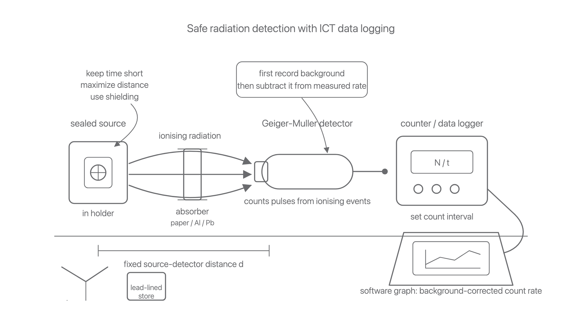
A common school detector is a Geiger-Muller tube connected to a counter, rate meter or data logger. Ionising radiation entering the detector can produce an electrical pulse. The counter records pulses as counts.
[DIAGRAM: asset_name: Lesson 1.02.2c: ICT, data logging and ionising radiation - diagram 01; asset_slug: 1_02_2c_ict_data_logging_and_ionising_radiation__diagram_01; recommended_method: drawn_physics; description: 16:9 apparatus layout on a white background showing a sealed radioactive source in a holder, absorber slot, fixed source-detector distance, Geiger-Muller detector connected to a counter/data logger and laptop graphing software. Include labels for background count, corrected count rate, count interval, absorber material, and safety controls such as tongs, shielding and source store.]
Several practical details matter:
- background radiation is always present, so measure background count rate first
- counts are random, so longer count intervals and repeated readings reduce the percentage random fluctuation in a mean count rate
- the source-detector distance and alignment must be fixed when comparing absorbers
- the detector window should face the source consistently
- the detector has limitations, so very high count rates or wrong geometry can give misleading data
- a simple GM detector counts ionising events but does not by itself identify the radiation type or energy
Corrected Count Rate
Here is number of counts and is the time interval. If the times are in seconds, the corrected rate is in count s.
Worked Example: correcting for background
A detector records 312 counts in 120 s with a source present. With the source removed and safely stored, it records 84 background counts in 180 s.
Source-present count rate:
Background count rate:
Corrected count rate:
The corrected rate is about to 2 significant figures. This is a count rate at the detector, not the source activity.
Safe Radiation Methods
Safe use is part of the outcome. A strong practical answer gives named precautions and links them to reducing exposure or improving data quality.
The core radiation safety ideas are:
- keep exposure time as short as reasonably possible
- keep as much distance as practical between people and the source
- use shielding, source holders and storage containers
- use the specified handling tool so that the source stays at least 10 cm from the hand; never touch it directly
- point the source away from people and return it to storage promptly
- follow local written instructions and teacher or technician supervision
PAG7-style work can involve observing the random nature of decay, comparing absorption by materials, or collecting counts over time for a half-life investigation. For this lesson, the common practical structure is the important part:
- Measure background count rate with no source in the measuring position.
- Place the sealed source in a holder.
- Align the detector at a fixed distance from the source.
- Choose a count interval long enough to reduce random fluctuation.
- Record counts for each condition, such as each absorber material or thickness.
- Repeat readings where possible and calculate mean corrected count rates.
- Keep the independent variable, dependent variable and control variables clear.
In an absorption investigation, the independent variable might be absorber material or absorber thickness. The dependent variable is the corrected count rate. Key control variables include source identity, source-detector distance and alignment, detector orientation, and absorber position. If material is the independent variable, absorber thickness should also be controlled. Equal count intervals are needed if raw counts are compared; count rates can be calculated from unequal intervals, although different intervals give different percentage random fluctuations.
Worked Example: count-rate calculation
A student records 320 counts in 40 s with a source present. The background count is 72 counts in 120 s.
Measured rate with source:
Background rate:
Corrected count rate:
Quick Check
Use this as a short comprehension check on the section above.
Practical Judgement
Many practical questions reward judgement. You may be asked to suggest equipment, justify a setting, improve a method, process readings, or evaluate whether the evidence justifies confidence in a conclusion.
For ICT and radiation-detector work, precise answers often use this pattern:
- identify the digital tool or detector
- state the measurement it records
- state the setting or control variable that matters
- explain how the data will be processed
- mention the main safety issue, uncertainty or limitation
For example, "use a data logger" is weak. A stronger answer is: "Use a GM tube connected to a counter or data logger; record counts for equal time intervals, subtract the background count rate, and compare corrected count rates with the source-detector distance and absorber position fixed."
Common traps are easy to avoid:
- do not say software improves accuracy unless you can name the error or limitation reduced
- do not process data without units
- do not ignore background radiation
- do not compare counts taken over different time intervals without converting to count rate
- do not treat a count-rate reading as source activity or dose without calibration
- do not describe unsafe handling of sources
Practical Judgement Summary
The skill is controlled practical use: digital tools collect and process data, while radiation detectors turn invisible ionising events into count data that must be corrected, repeated, controlled and collected safely.