3.1.2(a)(i) - Constant-acceleration equations
Constant acceleration is one of the most useful ideal models in mechanics. In this lesson you will connect the four constant-acceleration equations to a straight-line velocity-time graph, choose the right equation from the quantities in a problem, and apply the same model to vertical free fall when air resistance is ignored. The equations may look familiar, but the marks usually come from using signs, units and assumptions carefully.
The constant-acceleration model
The equations in this lesson apply to motion in a straight line with constant acceleration. That means the velocity changes by the same amount in each second.
Constant acceleration
Constant acceleration means that the acceleration has the same magnitude and direction throughout the time interval being modelled.
Use one sign convention along the line of motion. For horizontal motion, you might choose the direction of travel as positive. For vertical motion, you might choose upward or downward as positive, but you must then keep all displacements, velocities and accelerations consistent with that choice.
The five quantities are often remembered as suvat, but the letters are only useful if you know what each one means.
| Symbol | Meaning | Common unit |
|---|---|---|
| displacement during the interval | m | |
| initial velocity | m s^-1 | |
| final velocity | m s^-1 | |
| constant acceleration | m s^-2 | |
| time taken | s |
The word displacement matters. If an object moves forward and then back, the displacement is not the total distance travelled. These equations use signed displacement from the start of the chosen interval to the end.
A safe setup for any calculation is:
- Choose a positive direction.
- List the known values with signs and units.
- Identify the unknown.
- Choose an equation containing those quantities.
- Substitute, calculate, and check that the answer makes physical sense.
The constant-acceleration equations are one-dimensional vector equations. A sign convention is part of the physics, not a cosmetic detail.
Where the equations come from
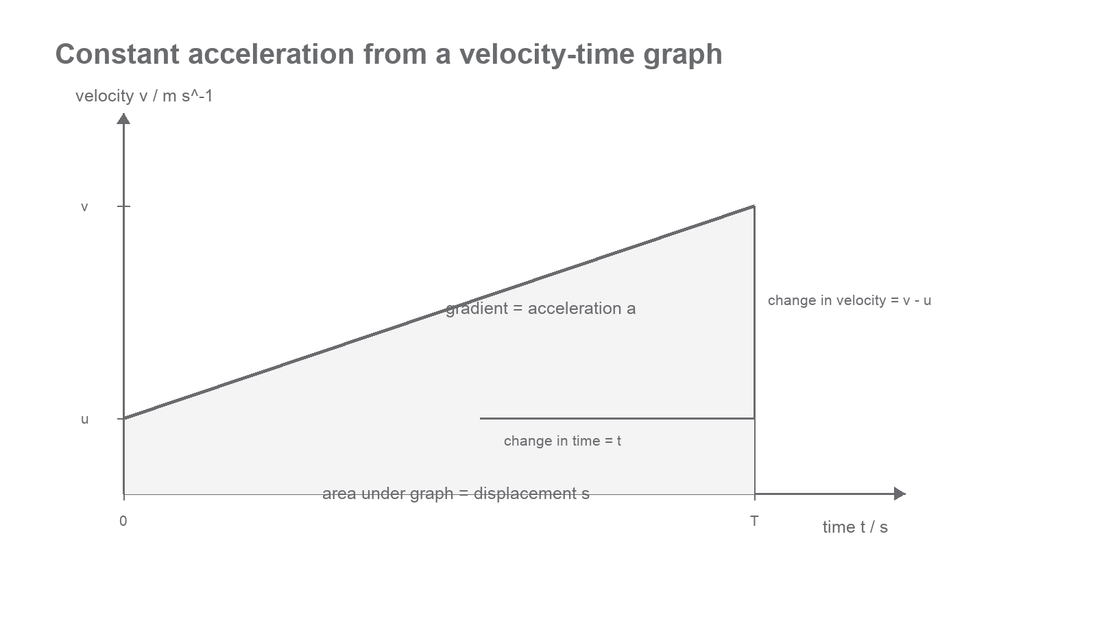
For constant acceleration, the velocity-time graph is a straight line. Its gradient is acceleration, its vertical intercept is the initial velocity, and the area under the graph is displacement.
[DIAGRAM: asset_name: Lesson 3.01.2a: Constant Acceleration Equations - diagram 01; asset_slug: 3_01_2a_constant_acceleration_equations__diagram_01; recommended_method: drawn_physics; description: A clean 16:9 velocity-time graph for constant acceleration with horizontal axis labelled time t / s and vertical axis labelled velocity v / m s^-1. Show a straight line from initial velocity u at t = 0 to final velocity v at t = T, label the intercept u, the final velocity v, the gradient a = (v - u) / t, and shade the trapezium under the line as displacement s. Use only #6A6B6E on white.]
From the gradient:
so:
Velocity after time
From the area under the velocity-time graph, the displacement is the area of a trapezium:
Displacement from average velocity
This equation works because, for constant acceleration, the average velocity is exactly:
Substitute into :
so:
Displacement from initial velocity
To remove time, combine with :
This rearranges to:
Velocity-displacement equation
These equations are given in the OCR data booklet, but the data booklet does not choose the equation, decide the signs or explain the model for you.
Choosing and rearranging an equation
Each constant-acceleration equation misses one of the five suvat quantities. That is the quickest way to choose.
| Equation | Quantity not used |
|---|---|
Worked example: final velocity and displacement
A trolley starts from and accelerates uniformly at for . Calculate its final velocity and displacement.
Known values:
Final velocity:
To calculate displacement without first rounding , use:
The data are mostly given to 2 significant figures, so a sensible final answer is:
Worked example: solving a quadratic time equation
A small vehicle is already moving at . It accelerates uniformly at . Calculate the time taken to travel a further .
Known values:
The final velocity is not given, so use:
Substitute:
Using the quadratic formula:
The negative time is not the time after the start of this interval, so reject it. The vehicle takes .
Free fall and sign conventions
In this lesson, free fall means motion under gravity with air resistance ignored. Near the Earth's surface, the acceleration of free fall has magnitude:
This value is given in the data booklet. The sign of the acceleration depends on your positive direction.
[DIAGRAM: asset_name: Lesson 3.01.2a: Constant Acceleration Equations - diagram 02; asset_slug: 3_01_2a_constant_acceleration_equations__diagram_02; recommended_method: drawn_physics; description: A clean 16:9 one-dimensional vertical free-fall sign convention diagram. Show a vertical axis labelled positive direction upward. Draw a ball moving upward with initial velocity arrow u upward, acceleration arrow a = -g downward, and a top point labelled v = 0 but a = -g still downward. Include a small note that choosing downward positive would make a = +g. Use only #6A6B6E on white.]
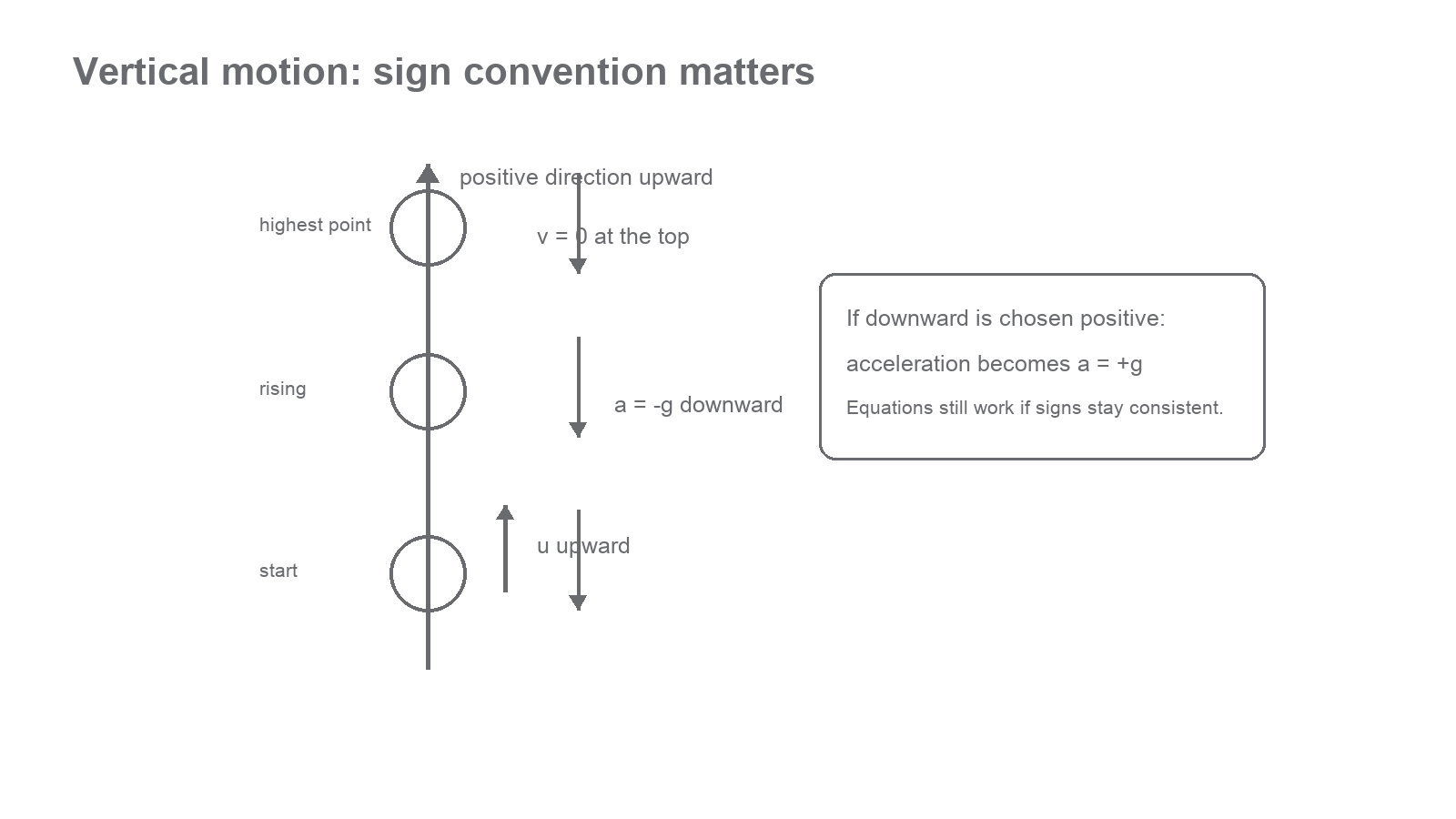
If upward is positive:
If downward is positive:
Both choices can be correct. Mixing the choices inside one calculation is not correct.
Worked example: dropped object
A small dense ball is dropped from rest through a vertical displacement of . Air resistance is negligible. Calculate the time taken and the final velocity just before it reaches the floor.
Choose downward as positive:
Use:
Since :
Now use :
Because downward was chosen as positive, this means downward. To 3 significant figures, and downward.
Worked example: object thrown upward
A ball is thrown vertically upward with initial velocity . Calculate the time to reach its highest point and the height gained. Ignore air resistance.
Choose upward as positive:
At the highest point the velocity is zero, but the acceleration is still downward.
For the time:
For the height:
The common error is to say acceleration is zero at the top because velocity is zero. That is wrong. Gravity is still changing the velocity at downward.
Limits and exam method
The equations are powerful because the model is simple. They are not a licence to ignore changing forces. If air resistance becomes significant, if an engine force changes, or if the object collides with something, acceleration may no longer be constant over the whole interval. Then these equations may apply only to a smaller part of the motion, or not at all.
For this lesson, the most important modelling assumption is:
Free fall without air resistance
Free fall without air resistance is motion where the only significant effect on the object is gravity, so the acceleration is constant and directed downward with magnitude .
In exam-style calculations, set out enough working for the method to be clear. A neat answer often has four lines:
- Known quantities with signs.
- Chosen equation.
- Substitution.
- Final answer with unit and sensible significant figures.
Worked example: choosing between two possible routes
A stone is moving downward at when it passes a window ledge. It then falls a further . Air resistance is negligible. Calculate its velocity after falling the .
Choose downward as positive:
Time is not needed, so use:
The stone is moving downward, so downward to 2 significant figures.