2.2.1 - Measurements and uncertainties
A physics measurement is not just a number. It is a number with a unit, a method, and a realistic statement of how much doubt is attached to it. In this lesson you will distinguish random and systematic errors, use precision and accuracy correctly, combine uncertainties in simple calculations, and use graph uncertainty to judge whether evidence supports a conclusion.
Measurement Errors
An error in measurement is the difference between a measured value and the true value. In real experiments the true value is usually not known exactly, so physicists describe likely error using uncertainty and by identifying the source of the error.
Random error
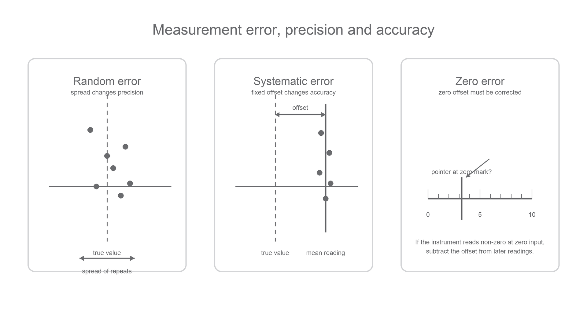
Random error causes repeated measurements of the same quantity to vary unpredictably about the best estimate. It affects the spread of readings.
Random error can come from reaction time, fluctuating readings, small changes in release position, reading a scale between marks, or environmental changes that are not fully controlled. Repeating measurements and calculating a mean can reduce the effect of random error because high and low readings partly balance.
Systematic error
Systematic error shifts measurements in the same direction from the true value. Repeating readings does not remove it.
Systematic error can come from a miscalibrated instrument, a scale read from the wrong zero, consistent parallax, a stopwatch started late in the same way each time, or an assumption in the method that is not valid.
Zero error
A zero error is a systematic error in which an instrument gives a non-zero reading when the quantity being measured is zero, or reads zero at the wrong position.
For example, if a digital balance reads +0.03 g when nothing is on it, every mass reading is likely to be too high by 0.03 g unless the balance is zeroed or the correction is applied. If a micrometer reads -0.02 mm when fully closed, a measured diameter must be corrected for that offset.
[DIAGRAM: asset_name: Lesson 2.02.1: Measurements, Errors And Uncertainties - diagram 01; asset_slug: 2_02_1_measurements_errors_and_uncertainties__diagram_01; recommended_method: drawn_physics; description: 16:9 NovaLearn-style deterministic diagram on a pure white background using only #6A6B6E. Three labelled panels: left panel shows repeated readings scattered around a vertical true value line labelled random error affects spread; centre panel shows repeated readings close together but shifted away from the true value line labelled systematic error affects accuracy; right panel shows an instrument scale with the pointer/display offset from zero labelled zero error correction. Include simple labels for true value, mean reading, spread, and zero offset.]
Worked example: correcting a zero error
A balance reads +0.04 g when there is no object on it. A metal washer then gives a displayed mass of 12.87 g.
The display is high by 0.04 g, so the corrected mass is:
The repeated display might be very steady, but the uncorrected value would still be inaccurate because the same offset is present in every reading.
Precision, Accuracy And Uncertainty
Precision and accuracy are not interchangeable.
Precision
Precision describes how closely repeated measurements agree with each other, or how finely a measuring instrument can resolve changes.
Accuracy
Accuracy describes how close a measured value is to the true value or an accepted value.
A set of readings can be precise but inaccurate. A mis-zeroed balance might give 12.87 g, 12.86 g, 12.87 g for the same object, so the readings are close together. If the balance has a zero error of +0.04 g, the uncorrected values are still too high.
Absolute uncertainty
Absolute uncertainty is the uncertainty written in the same unit as the measured quantity, such as 0.245 m +/- 0.002 m or 4.80 s +/- 0.05 s.
Percentage uncertainty
Percentage uncertainty is the absolute uncertainty expressed as a percentage of the measured value.
Percentage Uncertainty
The percentage uncertainty tells you whether the doubt is large compared with the measurement. An uncertainty of 0.5 mm is small for a length of 1.000 m, but large for a thickness of 2.0 mm.
Worked example: absolute and percentage uncertainty
A metre rule measurement is recorded as:
The absolute uncertainty is 0.001 m. The percentage uncertainty is:
A suitable statement is:
with percentage uncertainty about 0.21%.
Worked example: a small measurement has a larger percentage uncertainty
A wire diameter is recorded as:
The percentage uncertainty is:
The absolute uncertainty looks small, but it is about 2.4% of the diameter. That is why small distances often need a micrometer or vernier/digital calipers rather than a ruler.
Combining Uncertainties
OCR expects simple uncertainty techniques when measured data are combined. A rigorous statistical treatment is not required here, so use the standard A-level rules below unless a question gives a different instruction.
| Operation | Simple uncertainty rule |
|---|---|
| addition | add absolute uncertainties |
| subtraction | add absolute uncertainties |
| multiplication | add percentage uncertainties |
| division | add percentage uncertainties |
| raising to a power | multiply the percentage uncertainty by the power |
The rule changes because adding and subtracting compare quantities in the same unit, while multiplying, dividing and powers scale quantities by factors.
Addition Or Subtraction
Here or , and means absolute uncertainty. Even for subtraction, the uncertainties add because either reading could be at the end of its possible range in the direction that makes the final value most uncertain.
Worked example: uncertainty in a difference
A length change is found from two ruler readings:
- final position =
48.7 cm +/- 0.1 cm - initial position =
12.4 cm +/- 0.1 cm
The change in length is:
The absolute uncertainty is:
So:
The percentage uncertainty in the change is:
For multiplication and division, first convert each absolute uncertainty into a percentage uncertainty, then add the percentages.
Multiplication Or Division
Worked example: uncertainty in resistance
A resistor has:
The resistance is:
Percentage uncertainty in :
Percentage uncertainty in :
For division, add the percentage uncertainties:
Convert back to an absolute uncertainty if needed:
A suitable final answer is:
For a power, multiply the percentage uncertainty by the power. A constant such as , 2, or 4 does not add uncertainty.
Power Rule
Worked example: uncertainty in an area
A circle has radius:
Percentage uncertainty in :
Area is , so the percentage uncertainty in is:
The constant is not a measured quantity, so it does not contribute uncertainty.
Graphical Uncertainties
Graphs are often the clearest way to show uncertainty because the uncertainty can be drawn around the data. An error bar shows the range of possible values for a plotted point. If the uncertainty is only in the vertical quantity, draw vertical error bars. If uncertainty is relevant in both quantities, horizontal and vertical error bars may both be needed.
Error bar
An error bar is a graphical representation of the uncertainty in a plotted value. It shows the range within which the value is expected to lie according to the uncertainty information used.
The line of best fit should represent the overall trend in the points. It should not join point to point. If the plotted points have error bars, more than one line may be consistent with the data.
Line of best fit
A line of best fit is the straight line or smooth curve that best represents the trend in the plotted data.
Worst acceptable line
A worst acceptable line is an extreme line that is still reasonably consistent with the plotted points and their error bars. It is used to estimate uncertainty in a gradient or intercept.
[DIAGRAM: asset_name: Lesson 2.02.1: Measurements, Errors And Uncertainties - diagram 02; asset_slug: 2_02_1_measurements_errors_and_uncertainties__diagram_02; recommended_method: drawn_physics; description: 16:9 NovaLearn-style deterministic graph on a pure white background using only #6A6B6E. Show axes labelled x / unit and y / unit, five plotted crosses with vertical error bars, a solid line of best fit, a dashed worst acceptable line passing through the error-bar region, a large gradient triangle on the best-fit line, and labels for best gradient, worst gradient, uncertainty in gradient equals absolute difference, and y-intercept from x = 0.]
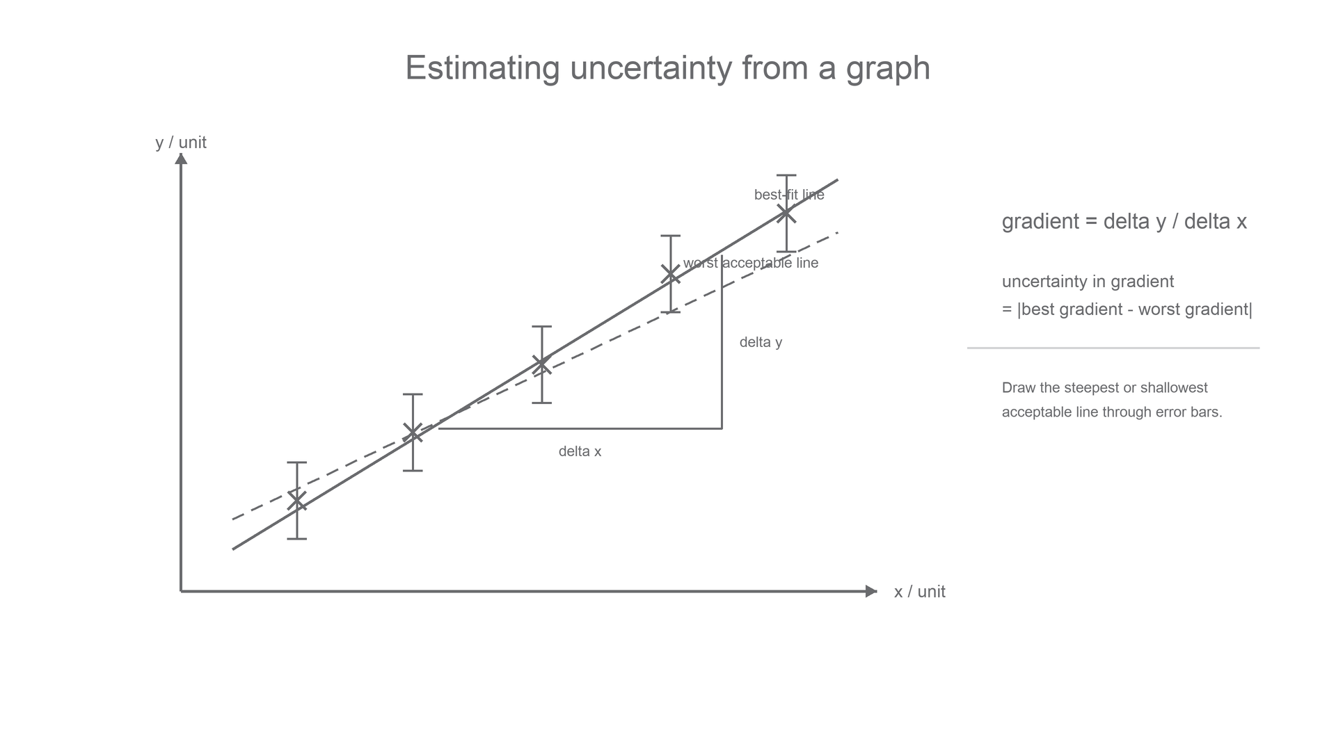
For a graph-based result, the uncertainty often comes from comparing the best-fit line with a worst acceptable line.
Gradient Uncertainty From A Worst Line
Similarly, if the intercept is important:
Here is gradient and is the vertical-axis intercept. The uncertainty is quoted as a positive value. If a specific exam question tells you to use a different comparison, follow the question, but this best-line versus worst-line method is a common OCR-style pattern.
Worked example: uncertainty in a graph gradient
A graph gives:
- best-fit gradient
- worst acceptable gradient
The absolute uncertainty in the gradient is:
So the result can be reported as:
The same idea works for an intercept. Use the difference between the best-fit intercept and the worst-line intercept, with the same unit as the vertical-axis quantity.
Graph uncertainty has a practical meaning. If the worst acceptable line gives a noticeably different gradient, the data do not support a very precise value. If the error bars are small and the worst line is close to the best-fit line, the graph supports a more precise gradient.
Percentage Difference And Judgement
Uncertainty calculations are only useful if they help you make a judgement. One common judgement is whether an experimental value agrees with an accepted value.
Percentage Difference
The modulus signs mean use the size of the difference, not whether it is positive or negative. A percentage difference does not explain the cause of the difference. It only tells you how far the experimental value is from the accepted value as a percentage of the accepted value.
Worked example: comparing with an accepted value
A student measures the acceleration of free fall as:
The accepted value is:
The uncertainty range is:
The accepted value lies inside this range, so the result is consistent with the accepted value within the uncertainty. The percentage difference is:
A good conclusion is:
"The measured value is 3.2% below the accepted value, but the accepted value lies inside the uncertainty range, so the experiment is consistent with the accepted value. The uncertainty is fairly large, so the result is not very precise."
Now compare this with:
The uncertainty range is 9.0 m s^-2 to 9.2 m s^-2, which does not include 9.81 m s^-2. This is a more serious disagreement. The measurements might be precise, but the result is inaccurate, so a systematic error or invalid assumption should be investigated.
When writing a final value with uncertainty, use compatible precision. For example:
- good:
0.58 +/- 0.05 ohm - good:
12.0 +/- 0.3 cm - poor:
0.583421 +/- 0.05 ohm - poor:
12.04 +/- 0.3 cm
The final value should not imply more precision than the uncertainty supports.
Percentage Difference And Judgement Summary
A strong measurement answer does three things: it identifies the kind of error, calculates uncertainty using the correct rule, and uses the uncertainty to make a justified conclusion.
Explain It Back
Use this as a self-explanation check after the section above. It is for diagnosing what you can already explain, not for learning new material from scratch.