1.3-1.5 - Distance-time graphs, speed and motion practical
Motion can be described with measurements instead of guesses. In this lesson, you will read and plot distance-time graphs, use average speed calculations, and plan a simple practical investigation using everyday objects such as toy cars or tennis balls. The key exam skill is linking the story of the motion to the numbers, units and graph shape.
What distance-time graphs show
A distance-time graph shows how far an object is from a starting point, or how much distance it has moved, at different times. Always read the axis label carefully, because an exam may use distance from start, distance travelled, or simply distance.
On a standard distance-time graph:
- time is on the horizontal axis
- distance is on the vertical axis
- each plotted point matches one time reading with one distance reading
Distance-time graph
A graph that shows the distance of an object at different times.
To plot one, choose sensible scales, plot points accurately with small crosses, and draw a straight line or smooth curve that represents the pattern. Do not join points with a jagged line unless the data genuinely shows abrupt changes. If a point does not fit the pattern, it may be anomalous, so think about whether it should be repeated or ignored.
The graph is not just a picture. It is a compact record of motion: the vertical change tells you how much the distance changed, and the horizontal change tells you how much time passed.
Explaining graph shape
The shape of a distance-time graph tells you how the motion changes.
A horizontal line means the distance is not changing. The object is stationary for that time interval.
A straight sloping line means the distance changes by equal amounts in equal times. The object is moving at constant speed.
A steeper line means a greater distance is covered in the same time. The speed is larger.
A curved line means the speed is changing. If the curve gets steeper, the object is speeding up. If it gets less steep, the object is slowing down. For this lesson, connect changing steepness to changing speed.
If the vertical axis is distance from start, a downward sloping line means the object is moving back towards the starting point. If the vertical axis is total distance travelled, the graph cannot go down, because total distance travelled only stays the same or increases.
Good graph explanations use interval language. Instead of saying "the graph goes up", say "from 0 s to 4 s the object moves away from the start at constant speed."
Average speed
Average speed tells you the distance moved per second, minute or hour over a whole journey or time interval. It does not say that the object moved at exactly that speed at every instant.
Average Speed
If distance is in metres and time is in seconds, the speed is in metres per second, written or . If distance is in kilometres and time is in hours, the speed is in kilometres per hour, written .
For example, a tennis ball moves in .
The formula can be rearranged if a different quantity is needed:
The distance in the formula is the total distance moved during the interval. If an object moves away from a start point and then returns, its final distance from the start is not the same as the total distance it moved.
Gradient is speed
For a straight section of a distance-time graph, the speed is the gradient of the line.
[DIAGRAM: asset_name: Distance-time graphs, speed and motion practical - diagram 01; asset_slug: p02_distance_time_graphs_speed_and_motion_practical__diagram_01; recommended_method: matplotlib; description: Monochrome 16:9 distance-time graph with axes time / s and distance from start / m. Plot a journey through points (0,0), (4,8), (7,8), (10,20), (13,8). Label sections constant speed, stationary, faster constant speed, and moving back toward start. Add a gradient triangle on the first section labelled change in distance = 8 m and change in time = 4 s.]
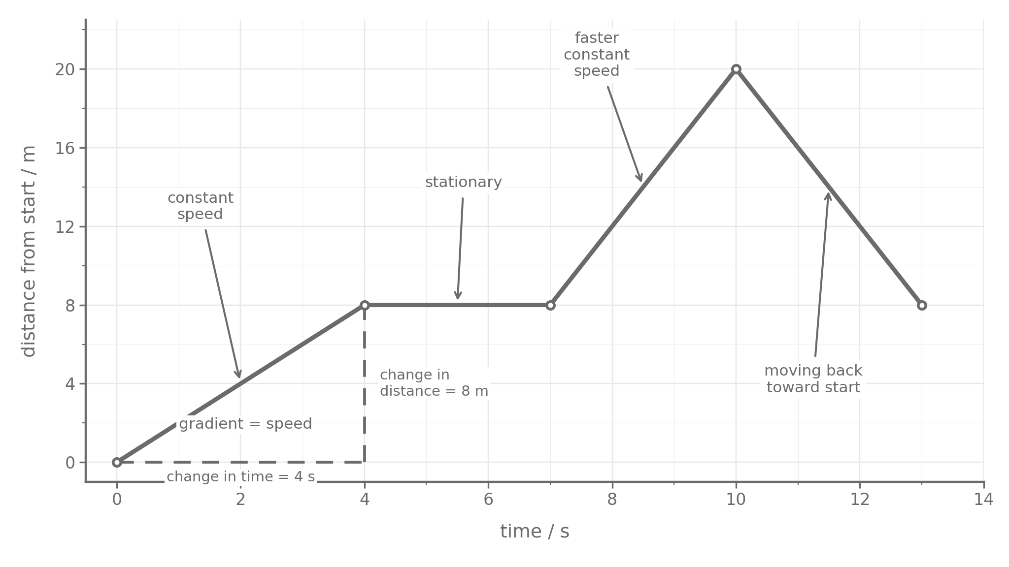
To calculate a gradient:
- Choose two clear points on the straight section.
- Find the change in distance between them.
- Find the change in time between them.
- Divide change in distance by change in time.
For the first sloping section in the diagram, the distance changes from to while the time changes from to .
For a curved graph, the speed is not constant. You can still compare speeds qualitatively by comparing steepness: the steeper part of the curve shows the greater speed.
Investigating motion
The required practical is to investigate the motion of everyday objects, such as toy cars or tennis balls. A simple method is to measure the time taken for an object to travel known distances, then use the data to calculate average speeds and plot a distance-time graph.
For a toy car:
- Set up a ramp or track and mark several distances along it, such as , , , and .
- Release the same toy car from the same starting position each time, without pushing it.
- Start timing when the front of the car passes the start mark.
- Stop timing when the front of the car reaches the chosen distance mark.
- Repeat each distance at least three times and calculate a mean time.
- Plot distance on the vertical axis against mean time on the horizontal axis.
For a tennis ball drop, the same measurement idea applies: measure a height or distance, time the motion, repeat, and use a consistent point on the ball when judging the start or finish.
The independent variable is the quantity you deliberately change, such as the distance mark or ramp height. The dependent variable is the quantity you measure, such as time taken or average speed. Control variables are kept the same, such as the toy car, release point, ramp surface and release method.
If the graph is a straight line through the data, the motion has constant speed over that range. If the graph curves, the speed is changing. If a car rolls down a ramp, it often speeds up, so one calculation of distance divided by time gives only the average speed for that whole run.
Improving and using data
Practical answers in Physics need more than "repeat it". You should be able to say what the main measurement problem is and how your method reduces it.
With stopwatch timing, human reaction time is often a large uncertainty. This matters most when the time interval is short. You can reduce its effect by using longer distances, repeating readings, using a clear start/finish marker, or using light gates or video analysis if available.
Distance measurements also need a consistent reference point. For a toy car, measure to the front of the car each time. For a ball, measure from the same part of the ball each time. Mixing reference points changes the measured distance and makes the results less valid.
A useful results table includes the distance, repeat times, mean time and calculated average speed:
| Distance in m | Time 1 in s | Time 2 in s | Time 3 in s | Mean time in s | Average speed in m/s |
|---|---|---|---|---|---|
| 0.40 | 0.88 | 0.84 | 0.86 | 0.86 | 0.47 |
| 0.80 | 1.30 | 1.34 | 1.32 | 1.32 | 0.61 |
| 1.20 | 1.66 | 1.70 | 1.68 | 1.68 | 0.71 |
The increasing average speed in this table suggests the car is not moving at constant speed over the measured runs. The data is more convincing because the repeat times are close together and the trend is consistent.
When evaluating a conclusion, link it to the evidence. "The car went faster" is weak. "The calculated average speed increased from to , so the car moved faster over the longer runs" is stronger because it quotes data.