The point-mapping idea

The safest way to transform a graph is to follow points. Suppose the point (p,q) lies on the graph y=f(x). That means

Each transformation tells you where the point (p,q) moves.

The outside of the function changes y-values. The inside of the function changes x-values. The inside rules feel reversed because the new x-value must make the inside input equal to the old x-value.

Worked example: the point P(4,-3) lies on y=f(x). Find the image of P on each transformed graph.

For y=f(x-2), the inside input is x-2. To use the old point at input 4, solve

so x=6. The y-value is unchanged, so

For y=f(2x), solve

so x=2. Again the y-value is unchanged, so

For y=3f(-x)+5, the inside -x gives

so x=-4. The outside part changes the y-value:

So

This point method also works for intercepts, stationary points, endpoints, and points on asymptotes.

Translations and stretches

A translation moves the whole graph without changing its shape. A stretch changes distances from an axis.

• y=f(x)+a is a vertical translation by a.
• y=f(x+a) is a horizontal translation by -a.
• y=af(x) is a vertical stretch by scale factor a; if a<0, this also reflects in the x-axis.
• y=f(ax) is a horizontal stretch by scale factor 1/a; if a<0, this also reflects in the y-axis.

For a sketch, transform a few reliable features first: roots, intercepts, stationary points, endpoints, and asymptotes. Then join them with the same kind of shape.

[DIAGRAM: asset_name: Lesson p1.2.9: Simple transformations of y = f(x) - diagram 01; asset_slug: p1_2_9_understand_the_effect_of_simple_transformations_on_the_graph_of_y_f_x__diagram_01; recommended_method: drawn_math; description: Draw the graph of a simple parabola y=f(x) and the transformed graph y=2f(3x) on the same axes. Use dashed styling for y=f(x) and solid styling for y=2f(3x). Mark corresponding points such as (-2,0)->(-2/3,0), (0,-2)->(0,-4), and (2,0)->(2/3,0). Label the point rule (p,q) -> (p/3,2q).]

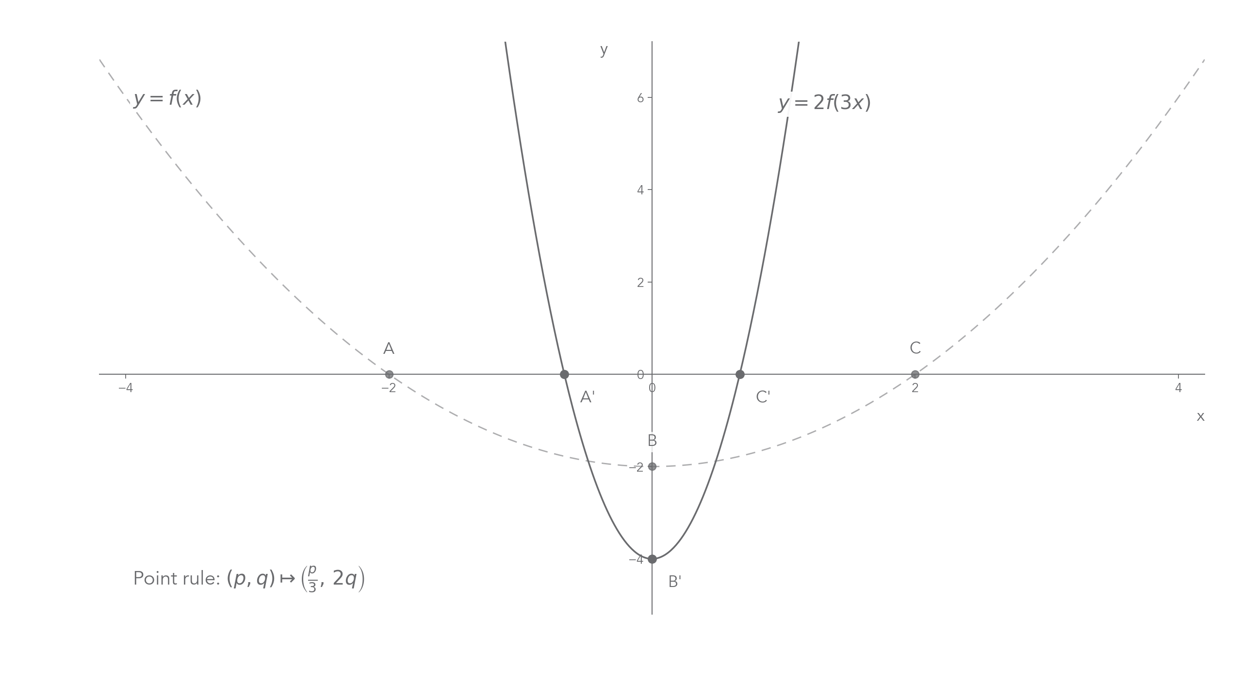
Worked example: a curve y=f(x) has key points

Find the corresponding points on y=2f(3x).

The inside transformation is 3x, so old x-coordinate p becomes p/3. The outside multiplier 2 means old y-coordinate q becomes 2q.

So

and

The graph is squeezed towards the y-axis by scale factor 1/3 and stretched vertically by scale factor 2.

Translations and stretches Continued

A useful check is to ask which axis is fixed. In y=af(x), points on the x-axis stay on the x-axis because a(0)=0. In y=f(ax), points on the y-axis stay on the y-axis because x=0 still gives input 0.

Modulus graphs

The graph y=|f(x)| takes every y-value on y=f(x) and makes it non-negative. Points already on or above the x-axis stay where they are. Points below the x-axis are reflected in the x-axis.

So if (p,q) lies on y=f(x), then on y=|f(x)| it becomes

Roots of f(x) stay fixed because |0|=0. Where the original graph crosses the x-axis, the modulus graph often has a sharp corner.

[DIAGRAM: asset_name: Lesson p1.2.9: Simple transformations of y = f(x) - diagram 02; asset_slug: p1_2_9_understand_the_effect_of_simple_transformations_on_the_graph_of_y_f_x__diagram_02; recommended_method: drawn_math; description: Draw two side-by-side panels. Left panel: show a cubic-like y=f(x) with parts below the x-axis, plus y=|f(x)| where the negative parts are reflected above the x-axis. Right panel: show y=|f(-x)|, making clear that the graph is first reflected in the y-axis and then folded above the x-axis. Mark roots and use direct labels without clutter.]

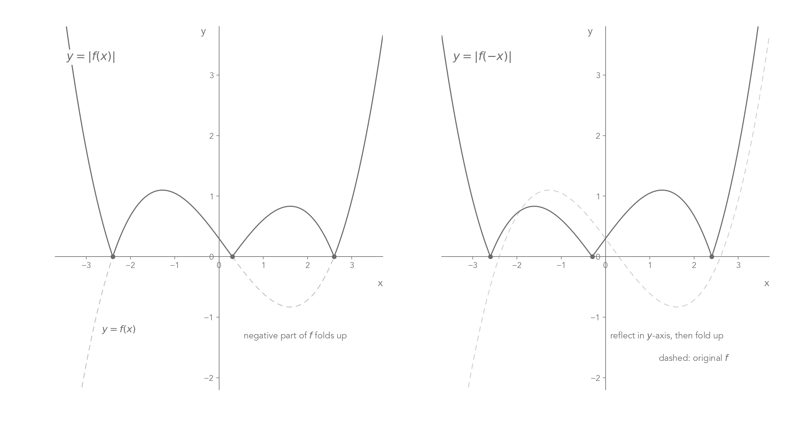
The graph y=|f(-x)| has two effects. The -x reflects the graph in the y-axis, and the modulus then folds any negative y-values above the x-axis. A point (p,q) on y=f(x) becomes

Worked example: suppose the graph y=f(x) has roots at x=-2 and x=4, and has a minimum point M(1,-3).

On y=|f(x)|, the roots stay at x=-2 and x=4, while

On y=|f(-x)|, reflect the x-coordinates first and make y-values non-negative. The roots become

and

Do not confuse |f(x)| with f(|x|). The first changes y-values; the second changes x-inputs. This lesson needs |f(x)| and |f(-x)|.

Combining transformations

For a combination, it is usually faster to use one point rule than to argue about the order in words.

If (p,q) lies on y=f(x), then on

where B != 0, the corresponding point is

This works because the new x-coordinate must make the inside input equal to the old x-coordinate:

Worked example: a curve y=f(x) has a maximum point A(-1,3) and a minimum point B(4,-2). Find the corresponding stationary points on

Here A=-2, B=2, C=-1, and D=3 in the general rule. For an old point (p,q),

and

For A(-1,3),

so A maps to (0,-3).

For B(4,-2),

so B maps to (5/2,7).

Because of the negative vertical multiplier, the old maximum becomes a minimum and the old minimum becomes a maximum.

Combining transformations Continued

One common wrong method is to multiply the x-coordinate by the number inside the bracket. For f(2x), the old x-coordinate is halved, not doubled. The input has to get to the same old value in half the x-distance.

Named function sketches

The same rules apply to any of the named A Level functions: quadratics, cubics, quartics, reciprocal graphs, trigonometric graphs, e^x, and a^x. The difference is that each family has its own features you should preserve or transform.

For polynomials, track roots, intercepts, and stationary points. For reciprocal graphs, track asymptotes as well as branches. For trigonometric graphs, track the midline, amplitude, period, and phase shift.

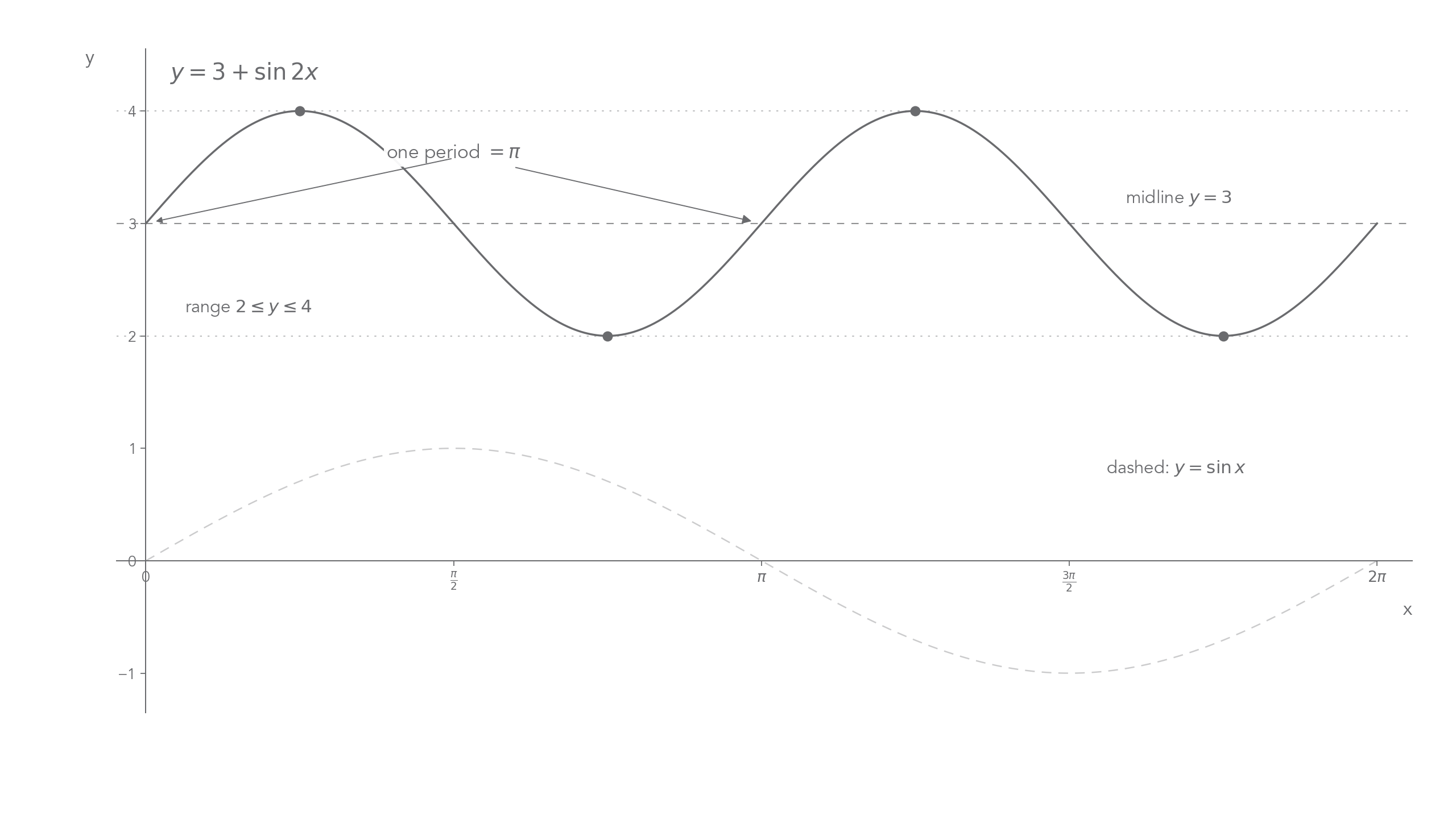
Worked example: sketch the key features of

from the graph of y=sin x.

The inside 2x halves the period:

The outside +3 translates the graph up by 3, so the midline is y=3. Since sin 2x still ranges from -1 to 1, the range is

On 0 <= x <= 2\pi, maxima occur when sin 2x=1, so

giving

Minima occur when sin 2x=-1, so

[DIAGRAM: asset_name: Lesson p1.2.9: Simple transformations of y = f(x) - diagram 03; asset_slug: p1_2_9_understand_the_effect_of_simple_transformations_on_the_graph_of_y_f_x__diagram_03; recommended_method: drawn_math; description: Draw y=3+sin 2x for 0 <= x <= 2pi, with the midline y=3, maximum level y=4, minimum level y=2, and one period length labelled as pi. Include a faint dashed reference curve y=sin x only if it remains uncluttered. Use exact tick labels 0, pi/2, pi, 3pi/2, 2pi.]

For a shifted and reflected cosine such as

the inside x+\pi/4 shifts the cosine graph left by \pi/4, and the outside negative sign reflects it in the x-axis. Its range is still -1<=y<=1, but maxima and minima swap compared with the shifted cosine.

Explain It Back

Use this as a self-explanation check after the section above. It is for diagnosing what you can already explain, not for learning new material from scratch.

When the question asks for a sketch, do not just write the transformation name. Mark enough transformed features for the graph to be unambiguous.