P1.2.11 - Functions in modelling
A function model turns a real situation into an equation that can be used for prediction and interpretation. In this lesson you will learn how to choose and use common function models, including trigonometric, exponential, and reciprocal models. You will also learn the Edexcel habit that matters just as much as calculation: every model has assumptions, a valid range, limitations, and possible refinements.
What a function model says
A function model uses one quantity as the input and predicts another quantity as the output. If the input is time t and the output is height H, then a model might be written as
The equation is not the real situation itself. It is a simplified rule that is useful only while its assumptions are reasonable.
Mathematical model
A mathematical model is a simplified mathematical description of a real situation. A function model gives a predicted output from an input, usually with constants that have contextual meanings.
When you read a function model, check four things.
| Feature | Question to ask |
|---|---|
| variables | What does each variable mean, and what are its units? |
| parameters | What do the constants mean in context? |
| domain | Which input values make sense in the situation? |
| assumptions | What has the model ignored or simplified? |
The contextual domain is often smaller than the mathematical domain. For example, the function T(t)=18+62e^{-0.08t} is mathematically defined for every real t, but if t means minutes after a cup of tea is poured, then t<0 does not belong to the model.
Worked example: interpreting a model.
The temperature, T degrees Celsius, of a drink t minutes after it is poured is modelled by
Find the initial temperature predicted by the model and interpret the number 18.
At the start, t=0, so
The model predicts an initial temperature of 80 degrees Celsius. The term 18 is the temperature the model approaches as t increases, so in context it represents the surrounding room temperature. It is not the initial temperature, because the exponential part is still present at t=0.
This example shows the key reading habit: substitute into the model, then interpret the result using the variables and units.
Choosing a function family
The specification expects you to recognise when a real situation is suited to a particular function family.
| Situation pattern | Useful function family | Typical model |
|---|---|---|
| repeated cycle such as tides or daylight | trigonometric | y=M+A cos(2*pi(t-h)/P) |
| constant percentage growth or decay | exponential | y=ab^t or y=ae^{kt} |
| inverse proportion | reciprocal | y=k/x |
The function family is chosen from the structure of the situation, not from a random curve-fitting instinct. A periodic quantity needs a periodic model. A quantity that changes by a constant percentage over equal time intervals suggests an exponential model. Two quantities whose product is constant suggest a reciprocal model.
[DIAGRAM: asset_name: Lesson p1.2.11: Functions as models, limitations, and refinements - diagram 01; asset_slug: p1_2_11_use_functions_in_modelling_and_appreciate_their_limitations_and_refinements__diagram_01; recommended_method: drawn_math; description: Draw three spacious coordinate panels. Panel 1: a trigonometric tide-style model D(t)=7+3cos(pi t/6) over 0<=t<=12, with maximum 10, minimum 4, midline D=7, and period 12 h labelled. Panel 2: an exponential decay model C(t)=20e^{-0.3t}, t>=0, with initial value 20 and horizontal asymptote C=0 labelled. Panel 3: a reciprocal inverse-proportion model P=240/V for V>0, with two labelled points showing PV=240 and the restriction V>0. Use direct labels, compact legends, axes, and clear margins.]
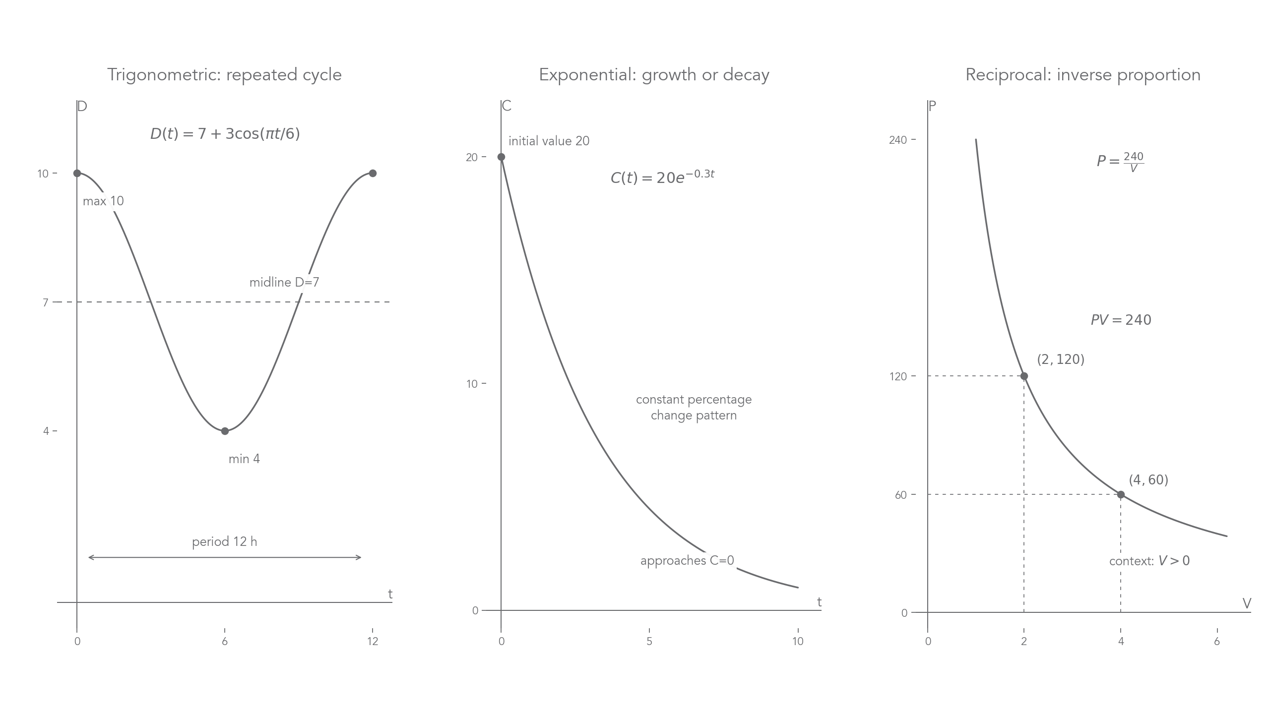
For a trigonometric model, a common form is
Here M is the midline, |A| is the amplitude, P is the period, and h shifts the cycle horizontally. The angle inside sin or cos is in radians, so the factor 2*pi/P gives one full cycle when t increases by P.
Worked example: modelling a tide.
At a harbour, high tide is 10 m at midnight, low tide is 4 m 6 hours later, and the next high tide is 12 hours after midnight. Write a simple cosine model for the depth D metres, t hours after midnight, for 0 <= t <= 12.
The midline is the average of the maximum and minimum:
The amplitude is half the range:
The period is 12 hours, so
Because the model starts at a maximum when t=0, cosine is convenient:
The model gives D(0)=10, D(6)=4, and D(12)=10, matching the information. A limitation is that real tides are not perfectly sinusoidal: wind, pressure, coastline shape, and later cycles may change the pattern.
Fitting constants and using a model
Many modelling questions give the form of the model and enough information to find its constants. The constants should be found from the data, kept with sensible accuracy, and then used for prediction.
For an exponential model
the constant p is the initial value because
The sign of k decides whether the model grows or decays. If k>0, the model grows. If k<0, the model decays.
Worked example: fitting an exponential decay model.
A machine is bought for 24000 pounds. Its value, V pounds, is modelled by
where t is the age of the machine in years. After 4 years, the value is 15000 pounds.
Find the model and use it to predict the value after 6 years.
At t=0,
so
Use the value after 4 years:
Divide by 24000:
Take natural logarithms:
so
The model is
An equivalent form is
After 6 years,
So the model predicts a value of about 11900 pounds to 3 significant figures.
The calculation is not finished until it is interpreted: the model predicts resale value, not exact market value. It ignores condition, mileage, supply, demand, and any minimum scrap value.
Limitations and validity
A model can be algebraically correct and still unsuitable for a particular prediction. In Edexcel modelling questions, you are often expected to comment on whether a prediction is reasonable.
Use these checks.
| Check | What it catches |
|---|---|
| contextual domain | input values that do not make sense, such as negative time |
| data range | extrapolation far outside the values used to build the model |
| output range | impossible predictions, such as negative mass or more than 100% |
| assumptions | ignored factors such as temperature, resistance, demand, or seasonal change |
| parameter meaning | constants that must stay fixed for the model to remain valid |
Interpolation and extrapolation
Interpolation uses a model between known data values. Extrapolation uses a model outside the known data range, so it is usually less reliable.
Worked example: using a reciprocal model critically.
For a fixed amount of gas at constant temperature, pressure P kPa and volume V litres are modelled by inverse proportion:
When V=3, the pressure is 80 kPa.
First find k:
So the model is
If V=2.4, then
The model predicts a pressure of 100 kPa.
Now consider the limitation. The model assumes the amount of gas and the temperature are constant, and it assumes the gas behaves ideally enough for inverse proportion to be reasonable. Also, V=0 is not allowed, and very small volumes may make the model physically unrealistic.
This is the difference between solving and modelling. Solving P=240/V is algebra. Deciding whether the prediction should be trusted is modelling.
Refining a model
To refine a model is to improve it after noticing a weakness. A refinement should be specific. Saying "make it more accurate" is too vague. A good refinement names what should change.
Common refinements include:
- restrict the domain of the model
- use a different function family
- add a vertical shift or limiting value
- include another variable that was ignored
- use more data to recalculate the constants
- split the situation into different time intervals with different models
Worked example: comparing and refining a cooling model.
A hot liquid has temperature 90 degrees Celsius at t=0. The room temperature is 20 degrees Celsius. Two possible models are considered:
and
where t is measured in minutes.
The linear model is simple, but it predicts
That is below room temperature. For a drink cooling in a room, this is not a reasonable long-term prediction.
The exponential model has a built-in limiting value:
As t increases, e^{-0.06t} gets closer to 0, so E(t) approaches 20. This better matches the assumption that the liquid cools towards room temperature.
A possible refinement would be to use more temperature readings to estimate the decay constant more accurately. Another possible refinement would be to change the limiting value if the room temperature changes.
Explain It Back
Use this as a self-explanation check after the section above. It is for diagnosing what you can already explain, not for learning new material from scratch.
The best modelling answers usually combine mathematics with context. They do not just say that a model is "bad". They explain which assumption fails, which input or output is outside the valid range, or which feature of the real situation is missing.