2.3.1 - Dijkstra's shortest-path algorithm
A route with the fewest links need not have the lowest cost. You will use Dijkstra's algorithm to keep track of the cheapest routes found so far, decide when a cost is final and recover the actual path. The edge weights, direction and tie rules will be explicit throughout.
A shortest path minimises total weight
A weighted graph assigns a cost to each edge, such as travel time or a fare. A path's cost is the sum of its edge weights. Here shortest means least total cost, not the fewest vertices, the fewest edges or the shortest line on a drawing.
If a direct edge P–R costs 12 but P–Q costs 3 and Q–R costs 4, the two-edge route costs 7 and is cheaper. All weights must measure the same quantity. Adding minutes to pounds would not define a meaningful route cost. In a directed graph, an edge P→Q permits that direction only; an undirected edge permits both directions with the stated weight.
Dijkstra's algorithm finds least-cost paths from one start vertex in a finite graph with non-negative weights. Zero is allowed. Negative edges break the finalisation argument used by this version. We assume every listed vertex exists, every edge endpoint is listed and every weight is a finite number. A missing edge means no direct connection; it does not mean a zero-cost connection.
For each vertex, store a tentative distance: the best cost from the start found so far. Initialise the start's distance to 0 and every other distance to infinity, meaning no route has yet been found. Also store a predecessor, initially none, to record the previous vertex on the best known route. No vertex is initially visited (finalised).
The frontier consists of unvisited vertices with finite tentative distances. Discovery puts a vertex on the frontier; it does not make its cost final. The start is initially the frontier's only member.
Choose the cheapest frontier vertex and relax edges
Each iteration selects the unvisited frontier vertex with the smallest tentative distance, then relaxes its edges to unvisited neighbours. Relaxing means testing whether a route through the selected vertex improves a neighbour's current record.
For a selected vertex u and neighbour v, calculate:
If the candidate is smaller than d(v), replace d(v) and set predecessor(v) to u. If it is larger, keep both records. In this lesson, an equal candidate also leaves the existing predecessor unchanged. That rule produces one reproducible least-cost path rather than storing all equally good paths.
Suppose B is selected with d(B)=3. D currently has distance 10, predecessor C, and B–D costs 5. The candidate is 3+5=8, so D becomes (8, B). If E currently has distance 7 and B–E costs 6, the candidate 9 is worse: E remains unchanged. Always add the start-to-B cost, not just the B–neighbour edge weight.
Mark the selected vertex visited. Its distance is now final: if a cheaper route to it existed, that route would have to pass from a previously visited region through an unvisited frontier vertex. That frontier cost is at least the selected minimum, and subsequent non-negative edges cannot reduce it. This is the reason for choosing the global frontier minimum, rather than following the cheapest edge out of the last vertex.
For equal minimum distances, we select the alphabetically first vertex. Another stated tie rule can change the visit order or chosen equal-cost path, but cannot change the minimum cost under these assumptions. Inspect neighbours alphabetically and update only on a strict improvement.
Trace distances and predecessors together
A trace must preserve both the current best costs and the decisions that changed them. Consider this original undirected graph, starting at A and aiming for F. Every edge is listed once; there are no other edges.
| Edge | Weight | Edge | Weight |
|---|---|---|---|
| A–B | 4 | A–C | 2 |
| B–C | 1 | B–D | 5 |
| C–D | 8 | C–E | 10 |
| D–E | 2 | D–F | 6 |
| E–F | 3 |
[DIAGRAM: Exact weighted connections of the A to F example; asset_slug: dijkstra-weighted-route; caption: Each labelled edge has the cost in the table. Line lengths do not represent costs.]
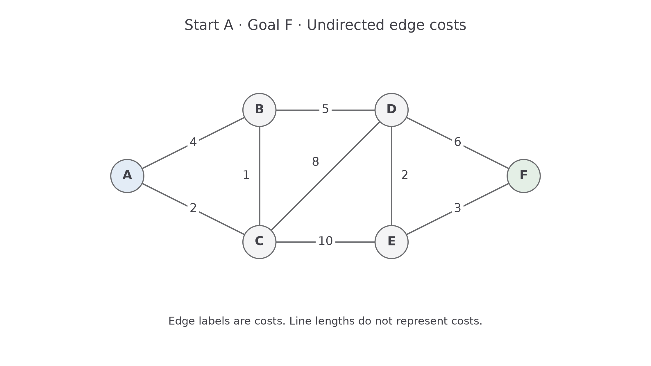
Write a record as vertex: distance / predecessor. A dash means no predecessor. The frontier is shown in increasing distance order; visited vertices have been removed from it. Initially A is 0 / –; B, C, D, E and F are infinity / –.
Continue this lesson.
You’re previewing NovaLearn without an account. Create a free account to read the rest.
Create free account