2.3.1 - A-star search and heuristics
A* combines the cost already spent with an estimate of the cost still needed. You will trace its open and closed sets, explain why a promising route is selected and identify the assumptions that let it return a shortest path. A useful estimate can save work, but its quality and the handling of revisits matter.
Combine travelled cost with estimated remaining cost
A-star (A*) searches a weighted graph for a least-cost route to a stated goal. Like Dijkstra's algorithm, it keeps the best discovered start-to-vertex cost and a predecessor. It also uses a heuristic, an estimate of the remaining cost from that vertex to the goal.
For a vertex n:
- g(n) is the best cost from the start found so far, using actual edge weights.
- h(n) is the supplied estimated remaining cost to the goal.
- f(n) is the estimated total cost of a route through n: .
A* selects the open vertex with the smallest f, not necessarily the smallest g or h alone. If P has g=4, h=8, then f=12. If Q has g=7, h=3, then f=10, so Q is selected first despite its more expensive journey so far. Selecting only h would be greedy best-first search and could ignore a large cost already incurred.
The estimates and edges must use compatible units. For travel time, a straight-line distance in kilometres cannot simply be added to minutes. Dividing that distance by a valid maximum travel speed could give a lower-bound time in compatible units. Straight-line distance is a useful distance heuristic only when route edge costs cannot be smaller than the corresponding direct geometric distances. A diagram's attractive layout does not establish that condition.
This lesson's main algorithm uses a finite graph, finite non-negative edge weights, a non-negative heuristic with h(goal)=0, and a consistent heuristic. Consistency means that for every permitted edge u→v of weight w,
For an undirected edge this must hold in both directions. Part 4 explains why this stronger condition matters for a version that never reopens closed vertices.
Maintain open records and close selected vertices
The open set is the frontier of discovered vertices still awaiting selection. The closed set contains selected vertices. Under the consistent-heuristic assumption, their g costs are final and this version does not reopen them.
Initially set g(start)=0, all other g values to infinity and all predecessors to none. Put only the start into open; closed is empty. Each iteration selects the open vertex with least f. Break an f tie alphabetically. Remove it from open and put it into closed. If it is the goal, return its g and recover the predecessor path; do not stop merely because a goal neighbour has been discovered.
Otherwise, inspect its outgoing edges to non-closed neighbours. For each neighbour v, compute candidate=g(u)+w(u,v). If this is strictly smaller than g(v), update g(v), predecessor(v)=u and f(v)=g(v)+h(v), and ensure v is in open. h(v) is the same supplied estimate; it does not become the edge weight or decrease because a better arrival route was found. Equal candidates keep the existing predecessor. Inspect neighbours alphabetically.
For example, R has g=5 and an edge of weight 2 to T. T currently has g=10, h=4 and predecessor P. The candidate is 7, so T becomes g=7, h=4, f=11, predecessor R. Forgetting to change its priority from 14 to 11 would allow the wrong next selection. Adding the edge to f(R), instead of g(R), would count an estimate as if it were an actual travelled cost.
The goal's h is zero, so its f equals its discovered route cost. Selection confirms that no better route remains under the stated safe heuristic/closed-set rules. If open becomes empty before the goal is selected, return no route. Start equal to goal returns cost 0 and the one-vertex path. Strict improvement and closed membership handle zero-cost edges without endlessly cycling.
Trace a route with a useful consistent heuristic
This original undirected graph starts at A and aims for F. The extra branch through X makes a comparison with Dijkstra meaningful. These are all its vertices and edges; positions in the picture do not define weights or heuristics.
| Edge | Weight | Edge | Weight |
|---|---|---|---|
| A–B | 4 | A–C | 2 |
| B–C | 1 | B–D | 5 |
| C–D | 8 | C–E | 10 |
| D–E | 2 | D–F | 6 |
| E–F | 3 | A–X | 1 |
| X–F | 30 |
| Vertex | A | B | C | D | E | F | X |
|---|---|---|---|---|---|---|---|
| h to F | 12 | 9 | 10 | 4 | 2 | 0 | 13 |
[DIAGRAM: Exact weighted graph and supplied heuristic labels for the A-star example; asset_slug: astar-weighted-heuristic; caption: Edge labels are actual costs. Node h labels are supplied remaining-cost estimates to F.]
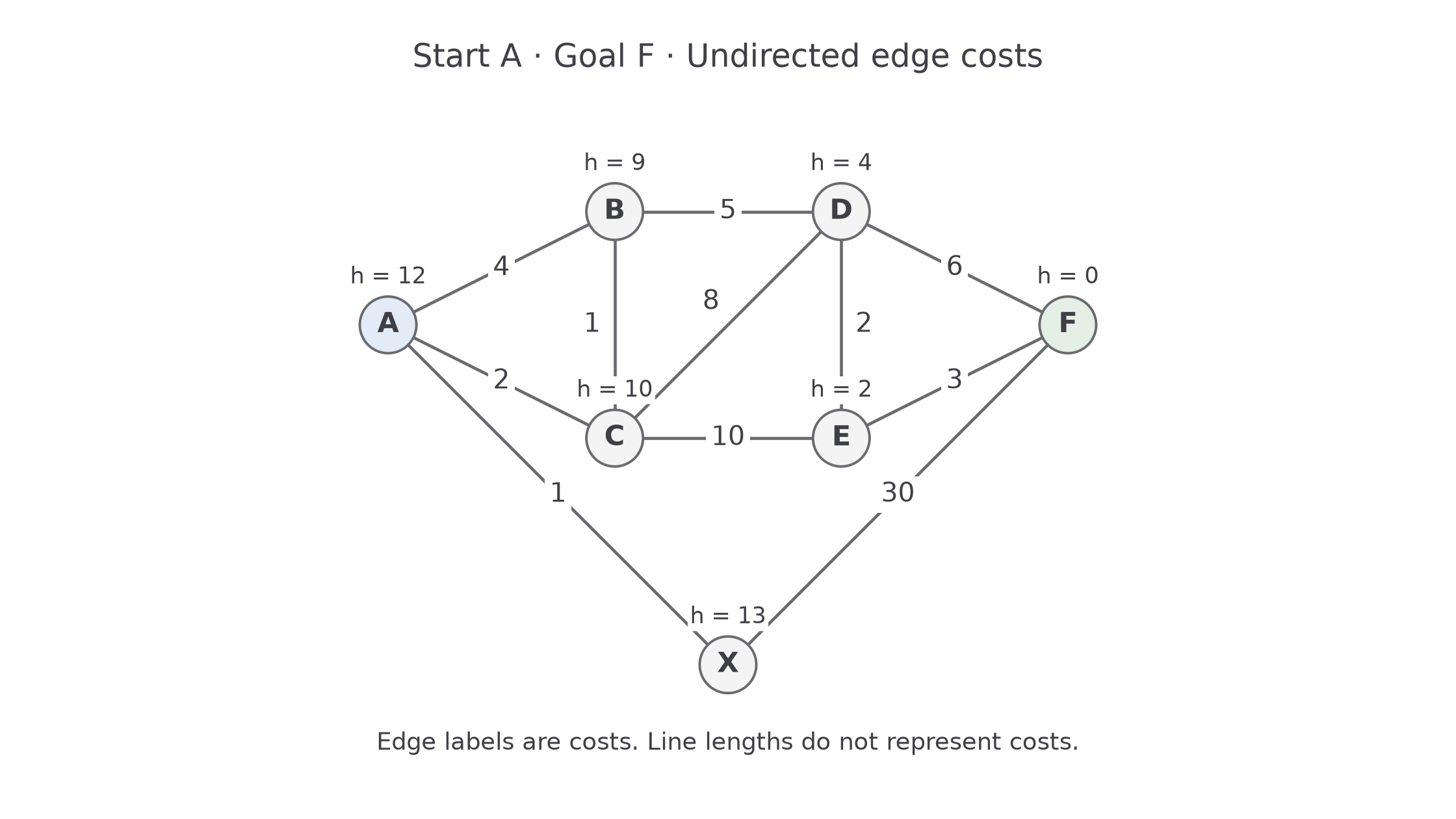
Write an open record as vertex: g,h,f / predecessor. All non-start g values are initially infinity. The start record is A:0,12,12/–. The open column below is ordered by f and then name; the closed column records selection order.
| Selected | Closed | Improvements made | Open after processing |
|---|---|---|---|
| A (f=12) | A | B:4/A; C:2/A; X:1/A | C:2,10,12/A; B:4,9,13/A; X:1,13,14/A |
| C (f=12) | A,C | B:3/C; D:10/C; E:12/C | B:3,9,12/C; D:10,4,14/C; E:12,2,14/C; X:1,13,14/A |
| B (f=12) | A,C,B | D:8/B | D:8,4,12/B; E:12,2,14/C; X:1,13,14/A |
| D (f=12) | A,C,B,D | E:10/D; F:14/D | E:10,2,12/D; F:14,0,14/D; X:1,13,14/A |
| E (f=12) | A,C,B,D,E | F:13/E | F:13,0,13/E; X:1,13,14/A |
| F (f=13) | A,C,B,D,E,F | Goal selected; stop | X:1,13,14/A |
Continue this lesson.
You’re previewing NovaLearn without an account. Create a free account to read the rest.
Create free account