4.2.3.2 - Distributions
A distribution reveals where scores cluster, how widely they vary and whether a tail pulls the pattern away from symmetry. You will distinguish normal, positive and negative skew, then predict the relative positions of mean, median and mode. Applying these features will help you interpret psychological data and select summaries while avoiding the common mistake of naming skew from where most scores, rather than the tail, appear.
What a distribution shows
Psychologists often collect a set of scores: memory test marks, reaction times, anxiety ratings, questionnaire totals or sleep hours. A distribution is the pattern those scores make when they are organised from low to high and counted.
Distribution
A distribution is the way scores or values are spread across a dataset.
Frequency
Frequency means how often a score, value or score interval occurs.
In this part of research methods, you are usually thinking about a frequency distribution: how many participants got each score, or how many scores fell into each interval. Recognising and sketching the shape both help you interpret where scores occur. Label score on the horizontal axis and frequency on the vertical axis; the height shows how common scores are, not how large an individual score is.
The shape of a distribution helps a researcher answer questions such as:
| Question about the data | What distribution shape can show |
|---|---|
| Are most scores around the middle? | The distribution may be normal or roughly symmetrical. |
| Are most scores bunched at one end? | The distribution may be skewed. |
| Are there a few unusually high or low scores? | These scores may pull the mean towards one tail. |
| Is one average likely to describe the data better than another? | Skew may make the median more useful than the mean for describing a typical score. |
A histogram of observed scores may approximate a smooth distribution curve. The curve describes the pattern of frequencies, while the score axis locates low and high values.
Normal distributions
In a normal distribution, scores form one symmetrical central peak.
Normal distribution
A normal distribution is a symmetrical, bell-shaped distribution in which most scores cluster around the centre and fewer scores occur at the extremes.
"Normal" does not mean morally normal, healthy or correct. It means the data follow a particular statistical pattern. Some psychological and biological variables are approximately normal in an appropriate population, although real datasets are rarely perfect. Increasing sample size does not turn an inherently skewed variable into a normal one.
A normal distribution has several key characteristics:
| Characteristic | What it means |
|---|---|
| Symmetrical shape | The left and right sides are mirror images, or very close to mirror images. |
| Bell shape | The distribution has one clear central peak and tapers away on both sides. |
| Central clustering | Most scores are close to the middle of the distribution. |
| Fewer extreme scores | Very low and very high scores are less frequent than middle scores. |
| Equal averages | The mean, median and mode are at the same central point in an ideal normal distribution. |
Measures of central tendency
Measures of central tendency are averages that summarise the centre or typical value of a dataset, such as the mean, median and mode.
The relationship between the mean, median and mode is useful because it gives a quick clue about shape. In a normal distribution, all three sit together at the centre:
| Measure | Position in a normal distribution |
|---|---|
| Mean | At the centre, because scores balance evenly on both sides. |
| Median | At the centre, because half the scores are below it and half are above it. |
| Mode | At the centre, because the most common score is around the peak. |
For an ideal normal distribution, approximately 68% of scores lie within one standard deviation of the mean, 95% within two, and 99.7% within three. These are areas under the curve, not heights at particular scores. For a mean of 100 and standard deviation of 15, about 68% lie between 85 and 115, about 95% between 70 and 130, and about 99.7% between 55 and 145. Roughly 2.5% lie above 130 and 2.5% below 70. Real data must be approximately normal before using these proportions.
Worked normal-area calculation
Suppose 200 scores are approximately normal with mean 50 and standard deviation 5. Two standard deviations is , so about 95% lie from 40 to 60. The remaining 5% is shared equally between the two tails: about 2.5%, or participants, lie above 60. Do not use 95% as the percentage below 60: that would omit the lower tail. These are approximate expectations, not guaranteed counts in a sample.
To sketch a normal distribution, draw one symmetric bell with equal tails tapering towards the score axis, and place the mean, median and mode together below the peak. A symmetric flat or two-peaked pattern is not normal just because its sides balance.
[DIAGRAM: asset_name: Normal distribution and central averages; asset_slug: 4_2_3_2_05_normal; description: An illustrative symmetric normal curve has one central peak, balanced tails and the mean, median and mode together at the centre.]
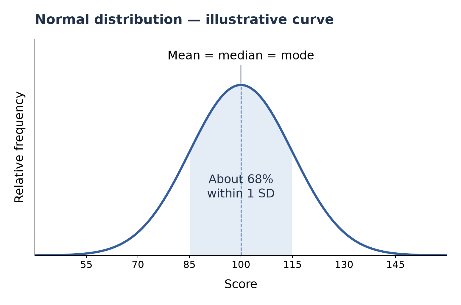
Example: A researcher gives a standardised attention test to 300 adults. Most people score near the average, with gradually fewer people scoring very low or very high. The left and right sides of the score pattern are roughly balanced. This would be described as an approximately normal distribution.
Be careful with the word "approximately". AQA questions may describe an ideal distribution, where the features are neat. Real psychological data can be messier, so it is better to say a dataset is roughly normal if it is broadly symmetrical and bell-shaped but not mathematically perfect.
Positive skew
Not all data are symmetrical. Sometimes scores are bunched at one end and stretch out towards the other end.
Skewed distribution
A skewed distribution is an asymmetrical distribution in which scores cluster more at one end and form a longer tail at the other end.
Tail
A tail is the thinner end of a distribution where fewer, more extreme scores occur.
The direction of skew is named after the direction of the tail, not the side where most scores are clustered. This is the detail students most often reverse.
Continue this lesson.
You’re previewing NovaLearn without an account. Create a free account to read the rest.
Create free account