2.2.3 - Digital sound
Specification point 2.2.3 turns a changing sound wave into a sequence a computer can store. You will connect amplitude, sample rate, sample interval and bit depth, then use those links to explain why two digital recordings can represent the same sound with different accuracy.
Analogue sound and amplitude
A microphone produces an electrical signal that changes as the sound changes. We can display this signal as a waveform:
- the horizontal axis represents time;
- the vertical axis represents amplitude;
- the centre line represents zero amplitude.
An analogue waveform is continuous. Between any two times, the signal can keep changing; it is not restricted to a fixed set of moments or heights.
Amplitude
Amplitude is the size of a sound wave, shown by its distance from the centre line on a waveform. A greater amplitude corresponds to a louder sound, all else being equal.
Suppose two claps are recorded with the same equipment. One waveform reaches an amplitude of 0.8 units while the other reaches 0.3 units. The first has the greater amplitude, so it represents the louder clap. The numbers here are illustrative measurements: they are not yet binary data.
When the sound is digitised, the computer does not store the whole continuous curve. It takes separate measurements of the waveform's amplitude. Each measurement is called a sample.
A sample records amplitude at one point in time. It does not measure the number of samples per second, and it is not a direct measurement of frequency.
This distinction lets us describe the waveform before deciding how often its amplitude will be measured.
Sampling in time
Digitising begins by choosing regular moments at which to measure the analogue waveform. Two linked quantities describe this timing.
Sample rate
Sample rate is the number of samples taken per second. It is measured in hertz (Hz), where 1 Hz means one sample per second.
Counting samples per second describes a rate. The gap between those samples is a duration instead.
Sample interval
Sample interval is the time between one sample and the next. It is measured in seconds.
For regular sampling, rate and interval are reciprocals:
sample interval (s) = 1 / sample rate (Hz)
sample rate (Hz) = 1 / sample interval (s)
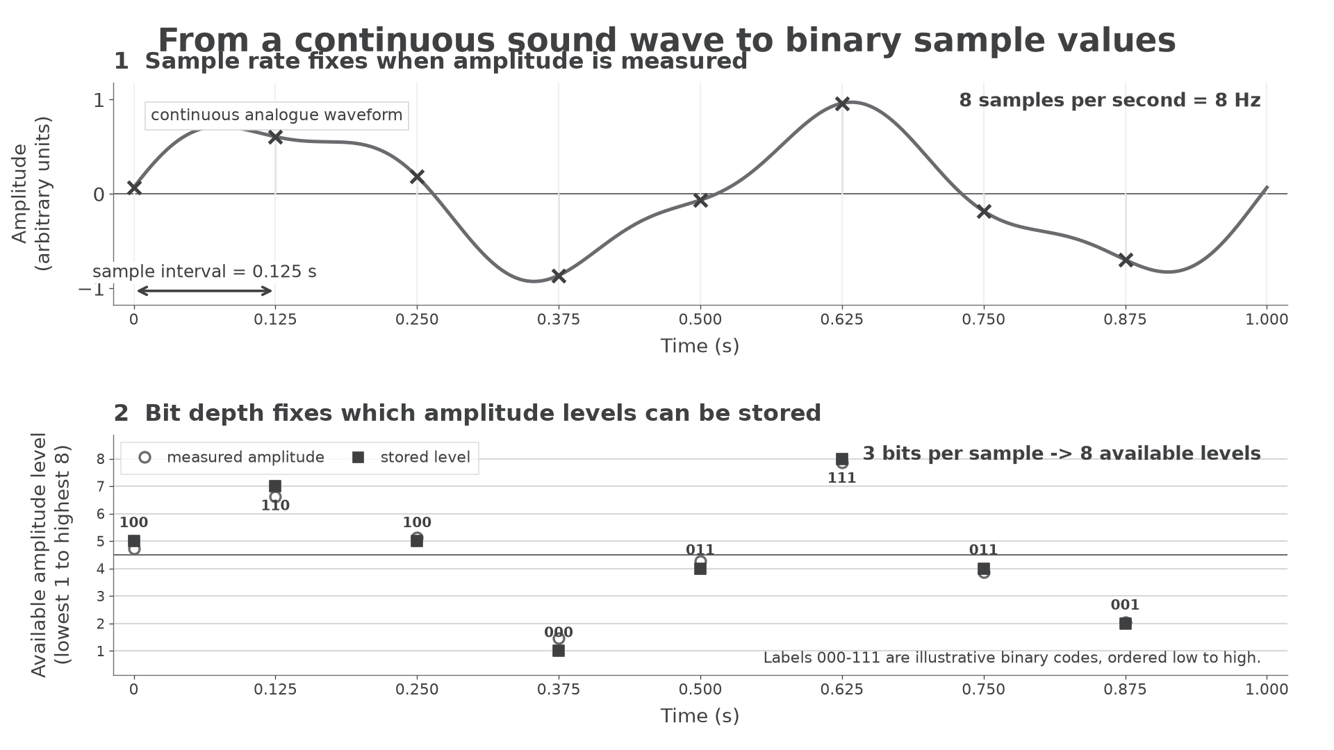
[DIAGRAM: asset_name: Sampling a sound wave in time and amplitude; asset_slug: 2_2_3_digital_sound__diagram_01; recommended_method: matplotlib; description: Exact two-panel monochrome quantitative plot. Top panel shows one continuous analogue waveform from 0 to 1 second sampled at eight evenly spaced times 0, 0.125, ..., 0.875 seconds, labelled sample rate 8 Hz and sample interval 0.125 s. Bottom panel shows those measured amplitudes rounded to eight horizontal levels for a 3-bit representation, with illustrative codes 000 to 111 ordered from lowest to highest; open circles are measured amplitudes, filled squares are stored levels, and dashed vertical gaps show rounding.]
Worked example: an 8 Hz recording
An 8 Hz sample rate means 8 samples per second.
sample interval = 1 / 8 s
                = 0.125 s
The samples in one second are therefore taken at 0, 0.125, 0.250, 0.375, 0.500, 0.625, 0.750 and 0.875 seconds. The moment 1.000 s begins the next one-second interval, so a sample there would be the next sample rather than a ninth sample inside the first interval.
If the rate doubles to 16 Hz, the interval halves:
sample interval = 1 / 16 s
                = 0.0625 s
The recorder now measures the waveform twice as often. More of its changes can be captured, so the digital representation can follow the original more closely.
Higher sample rate -> shorter sample interval -> more measurements each second. A larger sample interval has the opposite effect.
The next check keeps the units visible so rate and interval cannot be swapped.
Bit depth and amplitude levels
Sampling decides when amplitude is measured. The measurement must then be stored as a finite binary value.
Bit depth
Bit depth is the number of bits used to represent each sound sample.
If a sample has a bit depth of 3, each stored sample contains exactly three bits. The eight possible three-bit codes, from 000 to 111, can represent eight available amplitude levels. The lower panel of the diagram uses an illustrative low-to-high assignment of these codes.
The measured amplitude will often fall between two available levels. The system chooses the nearest level and stores that level's binary code. This rounding to an available level is called quantisation. The difference between the measured amplitude and the stored level is quantisation error.
Worked example: choosing a stored level
Suppose an amplitude measurement lies closest to the seventh of eight levels. With the diagram's illustrative low-to-high coding, the seventh level has code 110, so the stored sample is:
measured amplitude -> nearest available level -> 110
It is the code for the nearest level that is stored, not the original continuous height.
Increasing the bit depth from 3 to 4 bits increases the available levels from 8 to 16. Across the same amplitude range, the levels can be closer together. A measured amplitude can therefore be rounded to a nearer level, reducing quantisation error and making each sample a more precise representation.
The trade-off is binary data: a 4-bit sample stores one more bit than a 3-bit sample. This lesson compares that data amount qualitatively; it does not calculate sound-file sizes.
From analogue wave to binary data
The complete representation process combines timing and amplitude precision:
- Start with the continuous analogue waveform.
- Use the sample rate to set evenly spaced sample times. The reciprocal sample interval is the gap between them.
- Measure the waveform's amplitude at each sample time.
- Use the bit depth to select the nearest available amplitude level.
- Store that level as a binary code containing the stated number of bits.
The result is discrete in two ways. There are separate sample times rather than every possible moment, and there are separate available amplitude levels rather than every possible height. A line drawn between plotted samples may help us see the pattern, but the computer stores the binary sample values, not that continuous joining line.
| Feature | Analogue waveform | Digital representation |
|---|---|---|
| Time | Can vary continuously | Measurements at separate sample times |
| Amplitude | Can take any value in its range | Rounded to one of the available levels |
| Stored form | Not a sequence of binary samples | One fixed-length binary code per sample |
Pearson's reference example for CD-quality sound uses a sample rate of 44.1 kHz (44,100 samples per second) and a bit depth of 16 bits. It is stereo, so it uses two channels. These are useful reference settings; no channel or file-size calculation is needed here.
Because a practical digital representation uses a finite sample rate and finite bit depth, it is an approximation of the continuously changing original. Increasing either setting can increase accuracy, but it also creates more binary data for the same duration: more samples are stored, more bits are stored per sample, or both.
Reasoning about accuracy
An exam explanation should link a changed setting to the representation, then to its effect. Naming the setting alone is not enough.
Worked comparison
Two recorders capture the same one-second sound:
| Setting | Recorder A | Recorder B |
|---|---|---|
| Sample rate | 8 Hz | 16 Hz |
| Sample interval | 0.125 s | 0.0625 s |
| Bit depth | 3 bits | 4 bits |
| Available levels | 8 | 16 |
Recorder B can represent the sound more accurately for two different reasons:
- Timing chain: its higher sample rate gives a shorter sample interval, so it measures more points in the same second and is less likely to miss changes between samples.
- Amplitude chain: its greater bit depth gives more available amplitude levels, so each measurement can be rounded to a closer level with less quantisation error.
Recorder B also produces more binary data for the same duration. That is a trade-off, not evidence that sample rate and bit depth mean the same thing.
Sample rate controls detail across time. Bit depth controls precision in amplitude. Both can improve accuracy, but by different mechanisms.
A complete comparison must name both mechanisms rather than using the vague claim that one recording is simply "better quality".