1.2.6 - Search and sorting algorithms
Finding one value and putting a whole list in order look simple until the list grows. This lesson will help you trace linear and binary search, follow bubble and merge sort, and explain exactly what each algorithm checks, swaps, splits or merges.
Linear search
A search tries to locate a particular item, called the target, in a collection of data. It does not put the data into a new order. A search may return the target's index (its numbered position) or report that the target is not present.
Linear search
A linear search checks each item in sequence, starting at one end, until it finds the target or reaches the end of the list.
Linear search works even when the values are not sorted. Its steps are:
- Start at the first item.
- Compare the current item with the target.
- If they match, report the current index and stop.
- If they do not match, move to the next item.
- If the end is reached without a match, report that the target was not found.
Worked trace: finding a room number
Search the unsorted list [42, 17, 63, 28, 51] for target 28. The indices start at 0.
| Comparison | Index checked | Value checked | Match? | Action |
|---|---|---|---|---|
| 1 | 0 | 42 | No | Move to index 1 |
| 2 | 1 | 17 | No | Move to index 2 |
| 3 | 2 | 63 | No | Move to index 3 |
| 4 | 3 | 28 | Yes | Report index 3 and stop |
The algorithm does not check 51, because it stops as soon as the target is found. If the target were 35, all five values would be checked before the algorithm reported not found.
Linear does not mean random: the search follows the list one item at a time in a fixed sequence.
Binary search
Linear search can move through any list, but binary search makes a different decision: it uses the ordering of the data to rule out one whole part of the remaining list.
Binary search
A binary search finds a target in an ordered list by checking the middle item and repeatedly discarding the half in which the target cannot occur.
The ordered-list requirement is essential. In an ascending list, a target smaller than the midpoint can only be to its left, while a larger target can only be to its right. That reasoning is not valid in an unsorted list.
For every trace in this lesson, choose the middle-left item when the current interval has two middle items:
- Treat the entire ordered list as the current search interval.
- Check the item at the middle index.
- If it equals the target, report its index and stop.
- If the target is smaller, discard the midpoint and everything to its right.
- If the target is larger, discard the midpoint and everything to its left.
- Repeat on the remaining interval. If no indices remain, report
not found.
Worked trace: target found
Search for 47 in this ascending list.
| Index | 0 | 1 | 2 | 3 | 4 | 5 | 6 | 7 | 8 |
|---|---|---|---|---|---|---|---|---|---|
| Value | 4 | 9 | 15 | 22 | 31 | 38 | 47 | 53 | 64 |
| Step | Current indices | Midpoint index | Midpoint value | Decision |
|---|---|---|---|---|
| 1 | 0 to 8 | 4 | 31 | 47 > 31, so discard indices 0 to 4 |
| 2 | 5 to 8 | 6 | 47 | Match: report index 6 and stop |
The second interval has four items, so indices 6 and 7 are the two central choices. The stated middle-left convention selects index 6.
Worked trace: target absent
For target 30 in [5, 12, 18, 27, 34, 46, 59, 71], the midpoint values are 27, then 46, then 34.
| Step | Current indices | Midpoint | Decision | Next indices |
|---|---|---|---|---|
| 1 | 0 to 7 | index 3, value 27 | 30 > 27 | 4 to 7 |
| 2 | 4 to 7 | index 5, value 46 | 30 < 46 | 4 to 4 |
| 3 | 4 to 4 | index 4, value 34 | 30 < 34 | 4 to 3: empty |
Once the lower bound is greater than the upper bound, no candidate remains, so the result is not found.
The midpoint is the middle position in the current interval, not half of the target value.
Bubble sort
A sort rearranges all the items into a chosen order, such as ascending numerical order. Bubble sort does this through repeated passes across one working list.
Bubble sort
Bubble sort repeatedly compares adjacent items and swaps them when they are in the wrong order, continuing through passes until the list is sorted.
For an ascending bubble sort:
- Compare the first pair of adjacent values.
- Swap them if the left value is greater than the right value.
- Move one position to the right and compare the next adjacent pair.
- Reaching the end completes one pass.
- Repeat passes. In the version traced here, a complete pass with no swaps confirms that the list is sorted and stops the algorithm.
Only the adjacent pair currently being compared may be swapped. Bubble sort does not scan the list and move any convenient pair.
Worked trace: one complete pass
Sort [7, 3, 5, 2] into ascending order. The first pass is shown one comparison at a time.
| Comparison | Adjacent values | Swap? | List after comparison |
|---|---|---|---|
| Start | - | - | [7, 3, 5, 2] |
| 1 | 7 and 3 | Yes | [3, 7, 5, 2] |
| 2 | 7 and 5 | Yes | [3, 5, 7, 2] |
| 3 | 7 and 2 | Yes | [3, 5, 2, 7] |
The first pass has placed the largest value, 7, at the high end. It has not sorted the whole list.
Worked trace: later passes
| Pass | Start of pass | End of pass | Any swaps? |
|---|---|---|---|
| 2 | [3, 5, 2, 7] | [3, 2, 5, 7] | Yes |
| 3 | [3, 2, 5, 7] | [2, 3, 5, 7] | Yes |
| 4 | [2, 3, 5, 7] | [2, 3, 5, 7] | No: stop |
Pass 4 changes nothing, so this version has evidence that the values are already in order.
Merge sort
Merge sort uses divide and conquer: divide one problem into smaller versions, solve those smaller versions, then combine their results. For a list, the dividing continues until every sublist contains one item. A one-item list is already ordered.
Merge sort
Merge sort repeatedly splits a list into smaller sublists, then merges ordered sublists until one fully sorted list remains.
The complete process has two distinct phases:
- Split: divide the list into halves, then divide each half again, until only one-item lists remain.
- Merge: combine neighbouring ordered sublists. Compare their first unmerged values, move the smaller value to the output, and repeat. When one sublist is empty, append the values left in the other sublist.
[DIAGRAM: asset_name: Merge sort split and merge hierarchy; asset_slug: 1_2_6_search_and_sorting_algorithms__diagram_01; recommended_method: image_gen; description: A monochrome 16:9 hierarchy for ascending merge sort on [8, 3, 6, 1, 7, 2, 5, 4]. The top list branches downward through two four-item groups and four two-item groups to eight singleton lists. Below the singleton row, arrows converge downward through sorted pairs [3, 8], [1, 6], [2, 7], [4, 5], then sorted four-item groups [1, 3, 6, 8] and [2, 4, 5, 7], ending at [1, 2, 3, 4, 5, 6, 7, 8]. Split and merge stages are clearly labelled, with no extra algorithms or efficiency notation.]
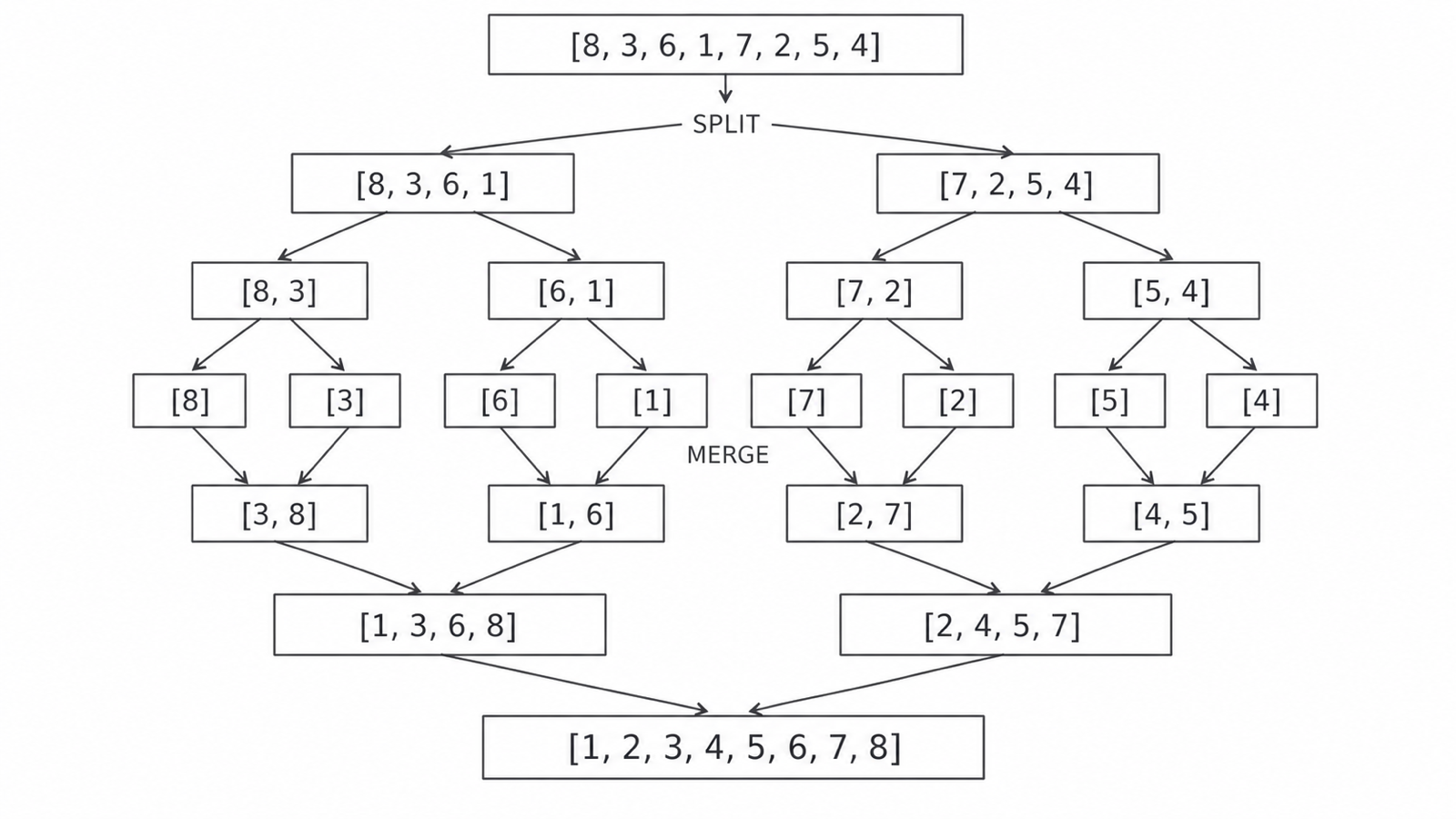
Worked trace: the split and merge states
Start with:
[8, 3, 6, 1, 7, 2, 5, 4]
Split into smaller groups:
[8, 3, 6, 1]    [7, 2, 5, 4]
[8, 3] [6, 1]    [7, 2] [5, 4]
[8] [3] [6] [1]  [7] [2] [5] [4]
Merge each neighbouring pair in ascending order:
[3, 8] [1, 6]    [2, 7] [4, 5]
[1, 3, 6, 8]     [2, 4, 5, 7]
[1, 2, 3, 4, 5, 6, 7, 8]
The last merge starts with ordered sublists [1, 3, 6, 8] and [2, 4, 5, 7]:
| Front values compared | Value moved to output | Output so far |
|---|---|---|
| 1 and 2 | 1 | [1] |
| 3 and 2 | 2 | [1, 2] |
| 3 and 4 | 3 | [1, 2, 3] |
| 6 and 4 | 4 | [1, 2, 3, 4] |
| 6 and 5 | 5 | [1, 2, 3, 4, 5] |
| 6 and 7 | 6 | [1, 2, 3, 4, 5, 6] |
| 8 and 7 | 7 | [1, 2, 3, 4, 5, 6, 7] |
The right sublist is now empty, so append the remaining 8 from the left sublist. Splitting alone has not sorted the data: the ordered result is created during the merge phase.
Tell the algorithms apart
The four algorithms solve two different kinds of problem. Linear and binary search try to locate one target; bubble and merge sort rearrange every item into order.
| Algorithm | Starting point | Repeated operation | Finishing result |
|---|---|---|---|
| Linear search | First item; data may be unsorted | Check the next item | Target found, or end reached |
| Binary search | Middle of an ordered interval | Compare, then discard the impossible half | Target found, or interval empty |
| Bubble sort | First adjacent pair in one working list | Compare and swap out-of-order neighbours through passes | A no-swap pass confirms the list is sorted |
| Merge sort | The whole unsorted list | Split to one-item lists, then merge ordered sublists | One ordered list remains |
The searches differ in where they look next: linear search advances by one item, while binary search uses the order to choose one half. The sorts differ in how they change the data: bubble sort performs adjacent swaps in repeated passes, while merge sort divides the list and then combines ordered groups.
Binary search and merge sort both show divide-and-conquer thinking because they repeatedly reduce a large problem to smaller parts. Binary search keeps only the one possible half; merge sort keeps all the parts and later combines them.
A binary search on unsorted data is not merely less effective; its decision about which half to discard is unreliable.